Ekman layer

The Ekman layer is the layer in a fluid where the flow is the result of a balance between pressure gradient, Coriolis and turbulent drag forces. In the picture above, the wind blowing North creates a surface stress and a resulting Ekman spiral is found below it in the column of water.

The Ekman layer is the layer in a fluid where there is a force balance between pressure gradient force, Coriolis force and turbulent drag. It was first described by Vagn Walfrid Ekman.

History

Ekman developed the theory of the Ekman layer after Fridtjof Nansen observed that ice drifts at an angle of 20°-40° to the right of the prevailing wind direction while on an Arctic expedition aboard the Fram. Nansen asked his colleague, Vilhelm Bjerknes to set one of his students upon study of the problem. Bjerknes tapped Ekman, who presented his results in 1902 as his doctoral thesis.^[1]

Mathematical formulation

The mathematical formulation of the Ekman layer can be found by assuming a neutrally stratified fluid, with horizontal momentum in balance between the forces of pressure gradient, Coriolis and turbulent drag.

{\begin{aligned}-fv&=-{\frac {1}{\rho _{o}}}{\frac {\partial p}{\partial x}}+K_{m}{\frac {\partial ^{2}u}{\partial z^{2}}},\\fu&=-{\frac {1}{\rho _{o}}}{\frac {\partial p}{\partial y}}+K_{m}{\frac {\partial ^{2}v}{\partial z^{2}}},\\0&=-{\frac {1}{\rho _{o}}}{\frac {\partial p}{\partial z}},\end{aligned}}

where $\ u$ and $\ v$ are the velocities in the $\ x$ and $\ y$ directions, respectively, $\ f$ is the local Coriolis parameter, and $\ K_{m}$ is the diffusive eddy viscosity, which can be derived using mixing length theory. Note that $p$ is a modified pressure: we have incorporated the hydrostatic of the pressure, to take account of gravity.

Boundary conditions

There are many regions where an Ekman layer is theoretically plausible; they include the bottom of the atmosphere, near the surface of the earth and ocean, the bottom of the ocean, near the sea floor and at the top of the ocean, near the air-water interface. Different boundary conditions are appropriate for each of these different situations. We will consider boundary conditions of the Ekman layer in the upper ocean:^[2]

{\text{at }}z=0:\quad A{\frac {\partial u}{\partial z}}=\tau ^{x}\quad {\text{and}}\quad A{\frac {\partial v}{\partial z}}=\tau ^{y},

where $\ \tau ^{x}$ and $\ \tau ^{y}$ are the components of the surface stress, $\ \tau$ , of the wind field or ice layer at the top of the ocean and $\ u_{g}$ and $\ v_{g}$ are the geostrophic flows in the $\ x$ and $\ y$ directions – as $\ z\to \infty :u\to u_{g},v\to v_{g}.$

In the other situations, other boundary conditions, such as the no-slip condition, may be appropriate instead.

Solution

Three views of the wind-driven Ekman layer at the surface of the ocean in the Northern Hemisphere. The geostrophic velocity is zero in this example.

These differential equations can be solved to find:

{\begin{aligned}u&=u_{g}+{\frac {{\sqrt {2}}}{fd}}e^{{z/d}}\left[\tau ^{x}\cos(z/d-\pi /4)-\tau ^{y}\sin(z/d-\pi /4)\right],\\v&=v_{g}+{\frac {{\sqrt {2}}}{fd}}e^{{z/d}}\left[\tau ^{x}\sin(z/d-\pi /4)+\tau ^{y}\cos(z/d-\pi /4)\right],\\d&={\sqrt {2K_{m}/f}}.\end{aligned}}

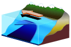
This variation of horizontal velocity with depth ( $-z$ ) is referred to as the Ekman spiral, diagrammed above and at right.

By applying the continuity equation we can have the vertical velocity as following

w={\frac {1}{f\rho _{o}}}\left[-\left({\frac {\partial \tau ^{x}}{\partial x}}+{\frac {\partial \tau ^{y}}{\partial y}}\right)e^{{z/d}}\sin(z/d)+\left({\frac {\partial \tau ^{y}}{\partial x}}-{\frac {\partial \tau ^{x}}{\partial y}}\right)(1-e^{{z/d}}\cos(z/d))\right].

Note that when vertically integrated the volume transport associated with the Ekman spiral is to the right of the wind direction in the Northern Hemisphere.

Experimental observations of the Ekman layer

There is much difficulty associated with observing the Ekman layer for two main reasons: the theory is too simplistic as it assumes a constant eddy viscosity, which Ekman himself anticipated,^[3] saying

“

It is obvious that

\ \left[\nu \right]

cannot generally be regarded as a constant when the density of water is not uniform within the region considered

”

and because it is difficult to design instruments with great enough sensitivity to observe the velocity profile in the ocean.

Laboratory demonstrations

The bottom Ekman layer can readily be observed in a rotating cylindrical tank of water by dropping in dye and changing the rotation rate slightly. Surface Ekman layers can also be observed in rotating tanks.

In the atmosphere

In the atmosphere, the Ekman solution generally overstates the magnitude of the horizontal wind field because it does not account for the velocity shear in the surface layer. Splitting the boundary layer into the surface layer and the Ekman layer generally yields more accurate results.^[4]

In the ocean

The Ekman layer, with its distinguishing feature the Ekman spiral, is rarely observed in the ocean. The Ekman layer near the surface of the ocean extends only about 10 – 20 meters deep,^[4] and instrumentation sensitive enough to observe a velocity profile in such a shallow depth has only been available since around 1980.^[2] Also, wind waves modify the flow near the surface, and make observations close to the surface rather difficult.^[5]

Instrumentation

Observations of the Ekman layer have only been possible since the development of robust surface moorings and sensitive current meters. Ekman himself developed a current meter to observe the spiral that bears his name, but was not successful.^[6] The Vector Measuring Current Meter ^[7] and the Acoustic Doppler Current Profiler are both used to measure current.

Observations

The first documented observations of an Ekman-like spiral were made in the Arctic Ocean from a drifting ice flow in 1958.^[8] More recent observations include:

The 1980 Mixed Layer Experiment^[9]
Within the Sargasso Sea during the 1982 Long Term Upper Ocean Study ^[10]
Within the California Current during the 1993 Eastern Boundary Current experiment ^[11]
Within the Drake Passage region of the Southern Ocean ^[12]
North of the Kerguelan Plateau during the 2008 SOFINE experiment ^[13]

Common to several of these observations spirals were found to be 'compressed', displaying larger estimates of eddy viscosity when considering the rate of rotation with depth than the eddy viscosity derived from considering the rate of decay of speed.^[10]^[11]^[12]^[13]

References

↑ Cushman-Roisin, Benoit (1994). "Chapter 5 - The Ekman Layer". Introduction to Geophysical Fluid Dynamics (1st ed.). Prentice Hall. pp. 76–77. ISBN 0-13-353301-8.
1 2 Vallis, Geoffrey K. (2006). "Chapter 2 – Effects of Rotation and Stratification". Atmospheric and Oceanic Fluid Dynamics (1st ed.). Cambridge, UK: Cambridge University Press. pp. 112–113. ISBN 0-521-84969-1.
↑ Ekman, V.W. (1905). "On the influence of the earth's rotation on ocean currents". Ark. Mat. Astron. Fys. 2 (11): 1–52.
1 2 Holton, James R. (2004). "Chapter 5 – The Planetary Boundary Layer". Dynamic Meteorology. International Geophysics Series. 88 (4th ed.). Burlington, MA: Elsevier Academic Press. pp. 129–130. ISBN 0-12-354015-1.
↑ Santala, M. J.; Terray, E. A. (1992). "A technique for making unbiased estimates of current shear from a wave-follower". Deep-Sea Research. 39 (3–4): 607–622. Bibcode:1992DSRI...39..607S. doi:10.1016/0198-0149(92)90091-7.
↑ Rudnick, Daniel (2003). "Observations of Momentum Transfer in the Upper Ocean: Did Ekman Get It Right?". Near-Boundary Processes and their Parameterization. Manoa, Hawaii: School of Ocean and Earth Science and Technology.
↑ Weller, R.A.; Davis, R.E. (1980). "A vector-measuring current meter". Deep-Sea Research. 27 (7): 565–582. Bibcode:1980DSRI...27..565W. doi:10.1016/0198-0149(80)90041-2.
↑ Hunkins, K. (1966). "Ekman drift currents in the Arctic Ocean". Deep-Sea Research. 13: 607–620. Bibcode:1966DSROA..13..607H. doi:10.1016/0011-7471(66)90592-4.
↑ Davis, R.E.; de Szoeke, R.; Niiler., P. (1981). "Part II: Modelling the mixed layer response". Deep-Sea Research. 28 (12): 1453–1475. Bibcode:1981DSRI...28.1453D. doi:10.1016/0198-0149(81)90092-3.
1 2 Price, J.F.; Weller, R.A.; Schudlich, R.R. (1987). "Wind-Driven Ocean Currents and Ekman Transport". Science. 238: 1534–1538. Bibcode:1987Sci...238.1534P. doi:10.1126/science.238.4833.1534.
1 2 Chereskin, T.K. (1995). "Direct evidence for an Ekman balance in the California Current". Journal of Geophysical Research. 100: 18261–18269. Bibcode:1995JGR...10018261C. doi:10.1029/95JC02182.
1 2 Lenn, Y; Chereskin, T.K. (2009). "Observation of Ekman Currents in the Southern Ocean". Journal of Physical Oceanography. 39: 768–779. Bibcode:2009JPO....39..768L. doi:10.1175/2008jpo3943.1.
1 2 Roach, C.J.; Phillips, H.E.; Bindoff, N.L.; Rintoul, S.R. (2015). "Detecting and Characterizing Ekman Currents in the Southern Ocean". Journal of Physical Oceanography. 45: 1205–1223. Bibcode:2015JPO....45.1205R. doi:10.1175/JPO-D-14-0115.1.

External links

Physical oceanography

Waves	Airy wave theory Ballantine scale Benjamin–Feir instability Boussinesq approximation Breaking wave Clapotis Cnoidal wave Cross sea Dispersion Edge wave Equatorial waves Fetch Gravity wave Green's law Infragravity wave Internal wave Kelvin wave Kinematic wave Longshore drift Luke's variational principle Mild-slope equation Radiation stress Rogue wave Rossby wave Rossby-gravity waves Sea state Seiche Significant wave height Sneaker wave Soliton Stokes boundary layer Stokes drift Stokes wave Swell Trochoidal wave Tsunami megatsunami Undertow Ursell number Wave action Wave base Wave height Wave power Wave radar Wave setup Wave shoaling Wave turbulence Wave–current interaction Waves and shallow water one-dimensional Saint-Venant equations shallow water equations Wind wave model

Circulation	Atmospheric circulation Baroclinity Boundary current Coriolis effect Downwelling Eddy Ekman layer Ekman spiral Ekman transport El Niño Southern Oscillation General Circulation Model Geostrophic current Global Ocean Data Analysis Project Gulf Stream Halothermal circulation Humboldt Current Hydrothermal circulation Langmuir circulation Longshore drift Loop Current Maelstrom Modular ocean model Ocean dynamics Ocean gyre Princeton ocean model Rip current Subsurface currents Sverdrup balance Thermohaline circulation shutdown Upwelling Whirlpool World Ocean Circulation Experiment

Tides	Amphidromic point Earth tide Head of tide Internal tide Lunitidal interval Perigean spring tide Rip tide Rule of twelfths Slack water Tidal bore Tidal force Tidal power Tidal race Tidal range Tidal resonance Tide gauge Tideline

Landforms	Abyssal fan Abyssal plain Atoll Bathymetric chart Coastal geography Cold seep Continental margin Continental rise Continental shelf Contourite Guyot Hydrography Oceanic basin Oceanic plateau Oceanic trench Passive margin Seabed Seamount Submarine canyon Submarine volcano

Plate tectonics	Convergent boundary Divergent boundary Fracture zone Hydrothermal vent Marine geology Mid-ocean ridge Mohorovičić discontinuity Vine–Matthews–Morley hypothesis Oceanic crust Outer trench swell Ridge push Seafloor spreading Slab pull Slab suction Slab window Subduction Transform fault Volcanic arc

Ocean zones	Benthic Deep ocean water Deep sea Littoral Mesopelagic Oceanic Pelagic Photic Surf

Sea level	Deep-ocean Assessment and Reporting of Tsunamis Future sea level Global Sea Level Observing System North West Shelf Operational Oceanographic System Sea-level curve Sea level rise World Geodetic System

Acoustics	Deep scattering layer Hydroacoustics Ocean acoustic tomography Sofar bomb SOFAR channel Underwater acoustics

Satellites	Jason-1 Jason-2 (Ocean Surface Topography Mission) Jason-3

Related	Argo Benthic lander Color of water DSV Alvin Marginal sea Marine energy Marine pollution Mooring National Oceanographic Data Center Ocean Ocean exploration Ocean observations Ocean reanalysis Ocean surface topography Ocean thermal energy conversion Oceanography Pelagic sediment Sea surface microlayer Sea surface temperature Seawater Science On a Sphere Thermocline Underwater glider Water column World Ocean Atlas

Category Commons

Authority control	GND: 4201370-7

This article is issued from Wikipedia - version of the 10/31/2016. The text is available under the Creative Commons Attribution/Share Alike but additional terms may apply for the media files.