Shallow water equations

Output from a shallow water equation model of water in a bathtub. The water experiences five splashes which generate surface gravity waves that propagate away from the splash locations and reflect off the bathtub walls.

The shallow water equations (also called Saint-Venant equations in its unidimensional form, after Adhémar Jean Claude Barré de Saint-Venant) are a set of hyperbolic partial differential equations (or parabolic if viscous shear is considered) that describe the flow below a pressure surface in a fluid (sometimes, but not necessarily, a free surface). The shallow water equations can also be simplified to the commonly used 1-D Saint-Venant equation.

The equations are derived^[1] from depth-integrating the Navier–Stokes equations, in the case where the horizontal length scale is much greater than the vertical length scale. Under this condition, conservation of mass implies that the vertical velocity of the fluid is small. It can be shown from the momentum equation that vertical pressure gradients are nearly hydrostatic, and that horizontal pressure gradients are due to the displacement of the pressure surface, implying that the horizontal velocity field is constant throughout the depth of the fluid. Vertically integrating allows the vertical velocity to be removed from the equations. The shallow water equations are thus derived.

While a vertical velocity term is not present in the shallow water equations, note that this velocity is not necessarily zero. This is an important distinction because, for example, the vertical velocity cannot be zero when the floor changes depth, and thus if it were zero only flat floors would be usable with the shallow water equations. Once a solution (i.e. the horizontal velocities and free surface displacement) has been found, the vertical velocity can be recovered via the continuity equation.

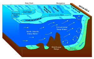
Situations in fluid dynamics where the horizontal length scale is much greater than the vertical length scale are common, so the shallow water equations are widely applicable. They are used with Coriolis forces in atmospheric and oceanic modeling, as a simplification of the primitive equations of atmospheric flow.

Shallow water equation models have only one vertical level, so they cannot directly encompass any factor that varies with height. However, in cases where the mean state is sufficiently simple, the vertical variations can be separated from the horizontal and several sets of shallow water equations can describe the state.

Equations

Conservative form

The shallow water equations are derived from equations of conservation of mass and conservation of linear momentum (the Navier–Stokes equations), which hold even when the assumptions of shallow water break down, such as across a hydraulic jump. In the case of no Coriolis, frictional or viscous forces, the shallow-water equations are:

${\begin{aligned}{\frac {\partial \eta }{\partial t}}+{\frac {\partial (\eta u)}{\partial x}}+{\frac {\partial (\eta v)}{\partial y}}&=0\\[3pt]{\frac {\partial (\eta u)}{\partial t}}+{\frac {\partial }{\partial x}}\left(\eta u^{2}+{\frac {1}{2}}g\eta ^{2}\right)+{\frac {\partial (\eta uv)}{\partial y}}&=0\\[3pt]{\frac {\partial (\eta v)}{\partial t}}+{\frac {\partial (\eta uv)}{\partial x}}+{\frac {\partial }{\partial y}}\left(\eta v^{2}+{\frac {1}{2}}g\eta ^{2}\right)&=0.\end{aligned}}$

Here η is the total fluid column height, and the 2D vector (u,v) is the fluid's horizontal velocity, averaged across the vertical column. g is acceleration due to gravity. The first equation is derived from mass conservation, the second two from momentum conservation.^[2]

Non-conservative form

Expanding the derivatives in the above using the product rule, we obtain non-conservative forms of the shallow-water equations. Since velocities are not subject to a fundamental conservation equation, the non-conservative forms do not hold across a shock or hydraulic jump. When we include also the appropriate terms for Coriolis, frictional and viscous forces, we obtain:

${\begin{aligned}{\frac {\partial u}{\partial t}}+u{\frac {\partial u}{\partial x}}+v{\frac {\partial u}{\partial y}}-fv&=-g{\frac {\partial h}{\partial x}}-bu,\\[3pt]{\frac {\partial v}{\partial t}}+u{\frac {\partial v}{\partial x}}+v{\frac {\partial v}{\partial y}}+fu&=-g{\frac {\partial h}{\partial y}}-bv,\\[3pt]{\frac {\partial h}{\partial t}}&=-{\frac {\partial }{\partial x}}{\Bigl (}u\left(H+h\right){\Bigr )}-{\frac {\partial }{\partial y}}{\Bigl (}v\left(H+h\right){\Bigr )},\end{aligned}}$

where

u	is the velocity in the x direction, or zonal velocity
v	is the velocity in the y direction, or meridional velocity
h	is the height deviation of the horizontal pressure surface from its mean height H
H	is the mean height of the horizontal pressure surface
g	is the acceleration due to gravity
f	is the Coriolis coefficient associated with the Coriolis force, on Earth equal to 2Ω sin(φ), where Ω is the angular rotation rate of the Earth (π/12 radians/hour), and φ is the latitude
b	is the viscous drag coefficient

It is often the case that the terms quadratic in u and v, which represent the effect of bulk advection, are small compared to the other terms. This is called geostrophic balance, and is equivalent to saying that the Rossby number is small. Assuming also that the wave height is very small compared to the mean height (h ≪ H), we have:

${\begin{aligned}{\frac {\partial u}{\partial t}}-fv&=-g{\frac {\partial h}{\partial x}}-bu,\\[3pt]{\frac {\partial v}{\partial t}}+fu&=-g{\frac {\partial h}{\partial y}}-bv,\\[3pt]{\frac {\partial h}{\partial t}}&=-H{\Bigl (}{\frac {\partial u}{\partial x}}+{\frac {\partial v}{\partial y}}{\Bigr )}\end{aligned}}$

One-dimensional Saint-Venant equations

The one-dimensional (1-D) Saint-Venant equations were derived by Adhémar Jean Claude Barré de Saint-Venant, and are commonly used to model transient open-channel flow and surface runoff. They can be viewed as a contraction of the two-dimensional (2-D) shallow water equations, which are also known as the two-dimensional Saint-Venant equations. The 1-D Saint-Venant equations contain to a certain extend the main characteristics of the channel cross-sectional shape.

The 1-D equations are used extensively in computer models such as HEC-RAS,^[3] SWMM5, ISIS,^[3] InfoWorks,^[3] Flood Modeller, SOBEK 1DFlow, MIKE 11,^[3] and MIKE SHE because they are significantly easier to solve than the full shallow water equations. Common applications of the 1-D Saint-Venant equations include flood routing along rivers (including evaluation of measures to reduce the risks of flooding), dam break analysis, storm pulses in an open channel, as well as storm runoff in overland flow.

The equations

Cross section of the open channel.

The system of partial differential equations which describe the 1-D incompressible flow in an open channel of arbitrary cross section – as derived and posed by Saint-Venant in his 1871 paper (equations 19 & 20) – are:^[4]

${\frac {\partial A}{\partial t}}+{\frac {\partial \left(Au\right)}{\partial x}}=0$ and

(1)

${\frac {\partial u}{\partial t}}+u\,{\frac {\partial u}{\partial x}}+g\,{\frac {\partial \zeta }{\partial x}}=-{\frac {P}{A}}\,{\frac {\tau }{\rho }},$

(2)

where x is the space coordinate along the channel axis, t denotes time, A(x,t) is the cross-sectional area of the flow at location x, u(x,t) is the flow velocity, ζ(x,t) is the free surface elevation and τ(x,t) is the wall shear stress along the wetted perimeter P(x,t) of the cross section at x. Further ρ is the (constant) fluid density and g is the gravitational acceleration.

Closure of the hyperbolic system of equations (1)–(2) is obtained from the geometry of cross sections – by providing a functional relationship between the cross-sectional area A and the surface elevation ζ at each position x. For example, for a rectangular cross section, with constant channel width B and channel bed elevation z_b, the cross sectional area is: A = B (ζ − z_b). The wall shear stress τ is dependent on the flow velocity u, they can be related by using e.g. the Darcy–Weisbach equation.

Further, equation (1) is the continuity equation, expressing conservation of water volume for this incompressible homogeneous fluid. Equation (2) is the momentum equation, giving the balance between forces and momentum change rates.

The instantaneous water depth is h(x,t) = ζ(x,t) − z_b(x), with z_b(x) the bed level (i.e. elevation of the lowest point in the bed above datum. The bed slope S(x), friction slope S_f(x,t) and hydraulic radius R(x,t) are defined as:

S=-{\frac {\mathrm {d} z_{\mathrm {b} }}{\mathrm {d} x}},

S_{\mathrm {f} }={\frac {\tau }{\rho gR}}

and

R={\frac {A}{P}}.

Consequently, the momentum equation (2) can be written as:^[5]

${\frac {\partial u}{\partial t}}+u\,{\frac {\partial u}{\partial x}}+g\,{\frac {\partial h}{\partial x}}+g\,\left(S_{\mathrm {f} }-S\right)=0.$

( 3)

Further note that – for non-moving channel walls – in the continuity equation (1): ∂A/∂t = B ∂ζ/∂t = B ∂h/∂t , with B(x,t) the momentary width of the free surface in the channel cross section at location x.^[5]

Equivalently, the momentum equation (3) can also be cast in the so-called conservation form, through some algebraic manipulations on the Saint-Venant equations, (1) and (3). In terms of the discharge Q = Au:^[6]

${\frac {\partial Q}{\partial t}}+{\frac {\partial }{\partial x}}\left({\frac {Q^{2}}{A}}+g\,I_{1}\right)+g\,A\,\left(S_{f}-S\right)-g\,I_{2}=0,$

( 4)

where A, I₁ and I₂ are functions of the channel geometry, described in the terms of the channel width B(σ,x). Here σ is the height above the lowest point in the cross section at location x, i.e. the height above the bed level z_b(x) (the lowest point in the cross section):

{\begin{aligned}A(\sigma ,x)&=\int _{0}^{\sigma }B(\sigma ^{\prime },x)\;\mathrm {d} \sigma ^{\prime },\\I_{1}(\sigma ,x)&=\int _{0}^{\sigma }(\sigma -\sigma ^{\prime })\,B(\sigma ^{\prime },x)\;\mathrm {d} \sigma ^{\prime }\qquad {\text{and}}\\I_{2}(\sigma ,x)&=\int _{0}^{\sigma }(\sigma -\sigma ^{\prime })\,{\frac {\partial B(\sigma ^{\prime },x)}{\partial x}}\;\mathrm {d} \sigma ^{\prime }.\end{aligned}}

Above – in the momentum equation (4) in conservation form – A, I₁ and I₂ are evaluated at σ = h(x,t). The term g I₁ describes the hydrostatic force in a certain cross section. And, for a non-prismatic channel, g I₂ gives the effects of geometry variations along the channel axis x.

In applications, depending on the problem at hand, there often is a preference for using either the momentum equation in non-conservation form, (2) or (3), or the conservation form (4). For instance in case of the description of hydraulic jumps, the conservation form is preferred since the momentum flux is continuous across the jump.

Characteristics

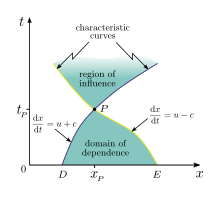
Characteristics, domain of dependence and region of influence, associated with location P = (x_P,t_P) in space x and time t.

The Saint-Venant equations (1)–(2) can be analysed using the method of characteristics.^[7]^[8]^[9]^[10] The two celerities dx/dt on the characteristic curves are:^[6]

{\frac {\mathrm {d} x}{\mathrm {d} t}}=u\pm c,

with

c={\sqrt {\frac {gA}{B}}}.

The Froude number F = |u| / c determines whether the flow is subcritical (F < 1) or supercritical (F > 1).

For a rectangular and prismatic channel of constant width B, i.e. with A = B h and c = √gh, the Riemann invariants are:^[7]

r_{+}=u+2{\sqrt {gh}}

and

r_{-}=u-2{\sqrt {gh}},

so the equations in characteristic form are:^[7]

{\begin{aligned}&{\frac {\mathrm {d} }{\mathrm {d} t}}\left(u+2{\sqrt {gh}}\right)=g\left(S-S_{f}\right)&&{\text{along}}\quad {\frac {\mathrm {d} x}{\mathrm {d} t}}=u+{\sqrt {gh}}\quad {\text{and}}\\&{\frac {\mathrm {d} }{\mathrm {d} t}}\left(u-2{\sqrt {gh}}\right)=g\left(S-S_{f}\right)&&{\text{along}}\quad {\frac {\mathrm {d} x}{\mathrm {d} t}}=u-{\sqrt {gh}}.\end{aligned}}

The Riemann invariants and method of characteristics for a prismatic channel of arbitrary cross-section are described by Didenkulova & Pelinovsky (2011).^[10]

The characteristics and Riemann invariants provide important information on the behavior of the flow, as well as that they may be used in the process of obtaining (analytical or numerical) solutions.

Derived modelling

Dynamic wave

The dynamic wave is the term used to describe the full 1-dimensional Saint-Venant equation. It is numerically challenging to solve, but is valid for all channel flow scenarios. The dynamic wave is used for modeling transient storms in modeling programs including HEC-RAS,^[11] InfoWorks,^[12] MIKE 11,^[13] Wash 123d ^[14] and SWMM.

Kinematic wave

For the kinematic wave it is assumed that the flow is uniform, and that the friction slope is approximately equal slope of the channel. This simplifies the full Saint-Venant equation to the kinematic wave:

S_{f}-S=0.

The kinematic wave is valid when the change in wave height over distance and velocity over distance and time is negligible relative to the bed slope, e.g. for shallow flows over steep slopes.^[15] The kinematic wave is used in HEC-HMS.^[16]

Diffusive wave

For the diffusive wave it is assumed that the inertial terms are less than the gravity, friction, and pressure terms. The diffusive wave can therefore be more accurately described as a non-inertia wave, and is written as:

g{\frac {\partial h}{\partial x}}+g(S_{f}-S)=0.

The diffusive wave is valid when the inertial acceleration is much smaller than all other forms of acceleration, or in other words when there is primarily subcritical flow. Models that use the diffusive wave assumption include MIKE SHE^[17] and LISFLOOD-FP.^[18]

Derivation from Navier–Stokes equations

The 1-D Saint-Venant momentum equation can be derived from the Navier–Stokes equations that describe fluid motion. The x-component of the Navier–Stokes equations – when expressed in Cartesian coordinates in the x-direction – can be written as:

{\frac {\partial u}{\partial t}}+u{\frac {\partial u}{\partial x}}+v{\frac {\partial u}{\partial y}}+w{\frac {\partial u}{\partial z}}=-{\frac {\partial p}{\partial x}}{\frac {1}{\rho }}+\nu \left({\frac {\partial ^{2}u}{\partial x^{2}}}+{\frac {\partial ^{2}u}{\partial y^{2}}}+{\frac {\partial ^{2}u}{\partial z^{2}}}\right)+f_{x},

where u is the velocity in the x-direction, v is the velocity in the y-direction, w is the velocity in the z-direction, t is time, p is the pressure, ρ is the density of water, ν is the kinematic viscosity, and f_x is the body force in the x-direction.

1.	If it is assumed that friction is taken into account as a body force, then ν can be assumed as zero so: $\nu \left({\frac {\partial ^{2}u}{\partial x^{2}}}+{\frac {\partial ^{2}u}{\partial y^{2}}}+{\frac {\partial ^{2}u}{\partial z^{2}}}\right)=0.$
2.	Assuming one-dimensional flow in the x-direction it follows that: $v{\frac {\partial u}{\partial y}}+w{\frac {\partial u}{\partial z}}=0$
3.	Assuming also that the pressure distribution is approximately hydrostatic it follows that: $p=\rho gh$ or in differential form: $\partial p=\rho g(\partial h).$ And when these assumptions are applied to the x-component of the Navier–Stokes equations: $-{\frac {\partial p}{\partial x}}{\frac {1}{\rho }}=-{\frac {1}{\rho }}{\frac {\rho g\left(\partial h\right)}{\partial x}}=-g{\frac {\partial h}{\partial x}}.$
4.	There are 2 body forces acting on the channel fluid, gravity, and friction: $f_{x}=f_{{x,g}}+f_{{x,f}}$ where f_x,g is the body force due to gravity and f_x,f is the body force due to friction.
5.	f_x,g can be calculated using basic physics and trigonometry: $F_{{g}}=(\sin \theta )gM$ where F_g is the force of gravity in the x-direction, θ is the angle, and M is the mass. Figure 1: Diagram of block moving down an inclined plane. The expression for sin θ can be simplified using trigonometry as: $\sin \theta ={\frac {\text{opp}}{\text{hyp}}}.$ For small θ (reasonable for almost all streams) it can be assumed that: $\sin \theta =\tan \theta ={\frac {\text{opp}}{\text{adj}}}=S$ and given that f_x represents a force per unit mass, the expression becomes: $f_{{x,g}}=gS.$
6.	Assuming the energy grade line is not the same as the channel slope, and for a reach of consistent slope there is a consistent friction loss, it follows that: $f_{{x,f}}=S_{f}g.$
7.	All of these assumptions combined arrives at the 1-dimensional Saint-Venant equation in the x-direction: ${\frac {\partial u}{\partial t}}+u{\frac {\partial u}{\partial x}}+g{\frac {\partial h}{\partial x}}+g(S_{f}-S)=0,$ $(a)\quad \ \ (b)\quad \ \ \ (c)\qquad \ \ \ (d)\quad (e)\$ where (a) is the local acceleration term, (b) is the convective acceleration term, (c) is the pressure gradient term, (d) is the friction term, and (e) is the gravity term.^[4]

Terms

The local acceleration (a) can also be thought of as the “unsteady term” as this describes some change in velocity over time. The convective acceleration (b) is an acceleration caused by some change in velocity over position, for example the speeding up or slowing down of a fluid entering a constriction or an opening, respectively. Both these terms make up the inertia terms of the 1-dimensional Saint-Venant equation.

The pressure gradient term (c) describes how pressure changes with position, and since the pressure is assumed hydrostatic, this is the change in head over position. The friction term (d) accounts for losses in energy due to friction, while the gravity term (e) is the acceleration due to bed slope.

Wave modelling by shallow water equations

Shallow water equations can be used to model Rossby and Kelvin waves in the atmosphere, rivers, lakes and oceans as well as gravity waves in a smaller domain (e.g. surface waves in a bath). In order for shallow water equations to be valid, the wavelength of the phenomenon they are supposed to model has to be much higher than the depth of the basin where the phenomenon takes place. Shallow water equations are especially suitable to model tides which have very large length scales (over hundred of kilometers). For tidal motion, even a very deep ocean may be considered as shallow as its depth will always be much smaller than the tidal wavelength.

Tsunami generation and propagation, as computed with the shallow water equations (red line; without frequency dispersion)), and with a Boussinesq-type model (blue line; with frequency dispersion). Observe that the Boussinesq-type model (blue line) forms a soliton with an oscillatory tail staying behind. The shallow water equations (red line) form a steep front, which will lead to bore formation, later on. The water depth is 100 meters.

Notes

↑ "The Shallow Water Equations" (PDF). Retrieved 2010-01-22.
↑ Clint Dawson and Christopher M. Mirabito (2008). "The Shallow Water Equations" (PDF). Retrieved 2013-03-28.
1 2 3 4 S. Néelz and G Pender (2009). "Desktop review of 2D hydraulic modelling packages". Joint Environment Agency/Defra Flood and Coastal Erosion Risk Management Research and Development Programme (Science Report: SC080035): p.5. Retrieved 2 December 2016. CS1 maint: Extra text (link)
1 2 Saint-Venant, A. J. C. Barré de (1871), Théorie du mouvement non permanent des eaux, avec application aux crues des rivières et a l’introduction de marées dans leurs lits. Comptes Rendus des Séances de l’Académie des Sciences, vol. 73, pp. 147–154 & 237–240.
1 2 Chow, Ven Te (1959), Open-channel hydraulics, McGraw-Hill, OCLC 4010975, §18-1 & §18-2.
1 2 Cunge, J. A., F. M. Holly Jr. and A. Verwey (1980), Practical aspects of computational river hydraulics, Pitman Publishing, ISBN 0 273 08442 9, §§2.1 & 2.2
1 2 3 Whitham, G. B. (1974) Linear and Nonlinear Waves, §§5.2 & 13.10, Wiley, ISBN 0-471-94090-9
↑ Lighthill, J. (2005), Waves in fluids, Cambridge University Press, ISBN 978-0-521-01045-0, §§2.8–2.14
↑ Meyer, R. E. (1960), Theory of characteristics of inviscid gas dynamics. In: Fluid Dynamics/Strömungsmechanik, Encyclopedia of Physics IX, Eds. S. Flügge & C. Truesdell ,Springer, Berlin, ISBN 978-3-642-45946-7, pp. 225–282
1 2 Didenkulova, I. and E. Pelinovsky (2011), Rogue waves in nonlinear hyperbolic systems (shallow-water framework), Nonlinearity 24(3), pp. R1–R18, doi:10.1088/0951-7715/24/3/R01
↑ Brunner, G. W. (1995), HEC-RAS River Analysis System. Hydraulic Reference Manual. Version 1.0 Rep., DTIC Document.
↑ Searby, D.; Dean, A.; Margetts J. (1998), Christchurch harbour Hydroworks modelling., Proceedings of the WAPUG Autumn meeting, Blackpool, UK.
↑ Havnø, K., M. Madsen, J. Dørge, and V. Singh (1995), MIKE 11-a generalized river modelling package, Computer models of watershed hydrology., 733–782.
↑ Yeh, G.; Cheng, J.; Lin, J.; Martin, W. (1995), A numerical model simulating water flow and contaminant and sediment transport in watershed systems of 1-D stream-river network, 2-D overland regime, and 3-D subsurface media . Computer models of watershed hydrology, 733–782.
↑ Novak, P., et al., Hydraulic Modelling – An Introduction: Principles, Methods and Applications. 2010: CRC Press.
↑ Scharffenberg, W. A., and M. J. Fleming (2006), Hydrologic Modeling System HEC-HMS: User's Manual, US Army Corps of Engineers, Hydrologic Engineering Center.
↑ DHI (Danish Hydraulic Institute) (2011), MIKE SHE User Manual Volume 2: Reference Guide, edited.
↑ Bates, P., T. Fewtrell, M. Trigg, and J. Neal (2008), LISFLOOD-FP user manual and technical note, code release 4.3. 6, University of Bristol.

External links

http://physics.nmt.edu/~raymond/classes/ph332/notes/shallowgov/shallowgov.pdf - derivation of the shallow water equations from first principles (instead of simplifying the Navier Stokes equations), some analytical solutions

Physical oceanography

Waves	Airy wave theory Ballantine scale Benjamin–Feir instability Boussinesq approximation Breaking wave Clapotis Cnoidal wave Cross sea Dispersion Edge wave Equatorial waves Fetch Gravity wave Green's law Infragravity wave Internal wave Kelvin wave Kinematic wave Longshore drift Luke's variational principle Mild-slope equation Radiation stress Rogue wave Rossby wave Rossby-gravity waves Sea state Seiche Significant wave height Sneaker wave Soliton Stokes boundary layer Stokes drift Stokes wave Swell Trochoidal wave Tsunami megatsunami Undertow Ursell number Wave action Wave base Wave height Wave power Wave radar Wave setup Wave shoaling Wave turbulence Wave–current interaction Waves and shallow water one-dimensional Saint-Venant equations shallow water equations Wind wave model

Circulation	Atmospheric circulation Baroclinity Boundary current Coriolis effect Downwelling Eddy Ekman layer Ekman spiral Ekman transport El Niño Southern Oscillation General Circulation Model Geostrophic current Global Ocean Data Analysis Project Gulf Stream Halothermal circulation Humboldt Current Hydrothermal circulation Langmuir circulation Longshore drift Loop Current Maelstrom Modular ocean model Ocean dynamics Ocean gyre Princeton ocean model Rip current Subsurface currents Sverdrup balance Thermohaline circulation shutdown Upwelling Whirlpool World Ocean Circulation Experiment

Tides	Amphidromic point Earth tide Head of tide Internal tide Lunitidal interval Perigean spring tide Rip tide Rule of twelfths Slack water Tidal bore Tidal force Tidal power Tidal race Tidal range Tidal resonance Tide gauge Tideline

Landforms	Abyssal fan Abyssal plain Atoll Bathymetric chart Coastal geography Cold seep Continental margin Continental rise Continental shelf Contourite Guyot Hydrography Oceanic basin Oceanic plateau Oceanic trench Passive margin Seabed Seamount Submarine canyon Submarine volcano

Plate tectonics	Convergent boundary Divergent boundary Fracture zone Hydrothermal vent Marine geology Mid-ocean ridge Mohorovičić discontinuity Vine–Matthews–Morley hypothesis Oceanic crust Outer trench swell Ridge push Seafloor spreading Slab pull Slab suction Slab window Subduction Transform fault Volcanic arc

Ocean zones	Benthic Deep ocean water Deep sea Littoral Mesopelagic Oceanic Pelagic Photic Surf Swash

Sea level	Deep-ocean Assessment and Reporting of Tsunamis Future sea level Global Sea Level Observing System North West Shelf Operational Oceanographic System Sea-level curve Sea level rise World Geodetic System

Acoustics	Deep scattering layer Hydroacoustics Ocean acoustic tomography Sofar bomb SOFAR channel Underwater acoustics

Satellites	Jason-1 Jason-2 (Ocean Surface Topography Mission) Jason-3

Related	Argo Benthic lander Color of water DSV Alvin Marginal sea Marine energy Marine pollution Mooring National Oceanographic Data Center Ocean Ocean exploration Ocean observations Ocean reanalysis Ocean surface topography Ocean thermal energy conversion Oceanography Pelagic sediment Sea surface microlayer Sea surface temperature Seawater Science On a Sphere Thermocline Underwater glider Water column World Ocean Atlas

Category Commons

This article is issued from Wikipedia - version of the 12/3/2016. The text is available under the Creative Commons Attribution/Share Alike but additional terms may apply for the media files.