Karyotype
A karyotype is the number and appearance of chromosomes in the nucleus of a eukaryotic cell. The term is also used for the complete set of chromosomes in a species or in an individual organism[1][2][3] and for a test that detects this complement or measures the number.
Karyotypes describe the chromosome count of an organism and what these chromosomes look like under a light microscope. Attention is paid to their length, the position of the centromeres, banding pattern, any differences between the sex chromosomes, and any other physical characteristics.[4] The preparation and study of karyotypes is part of cytogenetics.
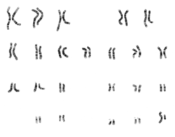
The study of whole sets of chromosomes is sometimes known as karyology. The chromosomes are depicted (by rearranging a photomicrograph) in a standard format known as a karyogram or idiogram: in pairs, ordered by size and position of centromere for chromosomes of the same size.
The basic number of chromosomes in the somatic cells of an individual or a species is called the somatic number and is designated 2n. Thus, in humans 2n = 46. In the germ-line (the sex cells) the chromosome number is n (humans: n = 23).[2]p28
So, in normal diploid organisms, autosomal chromosomes are present in two copies. There may, or may not, be sex chromosomes. Polyploid cells have multiple copies of chromosomes and haploid cells have single copies.
The study of karyotypes is important for cell biology and genetics, and the results may be used in evolutionary biology (karyosystematics)[5] and medicine. Karyotypes can be used for many purposes; such as to study chromosomal aberrations, cellular function, taxonomic relationships, and to gather information about past evolutionary events.
History of karyotype studies
Chromosomes were first observed in plant cells by Carl Wilhelm von Nägeli in 1842. Their behavior in animal (salamander) cells was described by Walther Flemming, the discoverer of mitosis, in 1882. The name was coined by another German anatomist, Heinrich von Waldeyer in 1888. It is New Latin from Ancient Greek κάρυον karyon, "kernel", "seed", or "nucleus", and τύπος typos, "general form").
The next stage took place after the development of genetics in the early 20th century, when it was appreciated that chromosomes (that can be observed by karyotype) were the carrier of genes. Grygorii Levitsky seems to have been the first person to define the karyotype as the phenotypic appearance of the somatic chromosomes, in contrast to their genic contents.[6][7] The subsequent history of the concept can be followed in the works of C. D. Darlington[8] and Michael JD White.[2][9]
Investigation into the human karyotype took many years to settle the most basic question: how many chromosomes does a normal diploid human cell contain?[10] In 1912, Hans von Winiwarter reported 47 chromosomes in spermatogonia and 48 in oogonia, concluding an XX/XO sex determination mechanism.[11] Painter in 1922 was not certain whether the diploid of humans was 46 or 48, at first favouring 46,[12] but revised his opinion from 46 to 48, and he correctly insisted on humans having an XX/XY system.[13] Considering the techniques of the time, these results were remarkable.
In textbooks, the number of human chromosomes remained at 48 for over thirty years. New techniques were needed to correct this error. Joe Hin Tjio working in Albert Levan's lab[14] was responsible for finding the approach:
- Using cells in tissue culture
- Pretreating cells in a hypotonic solution, which swells them and spreads the chromosomes
- Arresting mitosis in metaphase by a solution of colchicine
- Squashing the preparation on the slide forcing the chromosomes into a single plane
- Cutting up a photomicrograph and arranging the result into an indisputable karyogram.
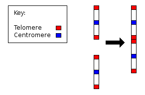
The work took place in 1955, and was published in 1956. The karyotype of humans includes only 46 chromosomes.[15][16] Rather interestingly, the great apes have 48 chromosomes. Human chromosome 2 is now known to be a result of an end-to-end fusion of two ancestral ape chromosomes.[17][18]
Observations on karyotypes
Staining
The study of karyotypes is made possible by staining. Usually, a suitable dye, such as Giemsa,[19] is applied after cells have been arrested during cell division by a solution of colchicine usually in metaphase or prometaphase when most condensed. In order for the Giemsa stain to adhere correctly, all chromosomal proteins must be digested and removed. For humans, white blood cells are used most frequently because they are easily induced to divide and grow in tissue culture.[20] Sometimes observations may be made on non-dividing (interphase) cells. The sex of an unborn fetus can be determined by observation of interphase cells (see amniotic centesis and Barr body).
Observations
Six different characteristics of karyotypes are usually observed and compared:[21]
- Differences in absolute sizes of chromosomes. Chromosomes can vary in absolute size by as much as twenty-fold between genera of the same family. For example, the legumes Lotus tenuis and Vicia faba each have six pairs of chromosomes, yet V. faba chromosomes are many times larger. These differences probably reflect different amounts of DNA duplication.
- Differences in the position of centromeres. These differences probably came about through translocations.
- Differences in relative size of chromosomes. These differences probably arose from segmental interchange of unequal lengths.
- Differences in basic number of chromosomes. These differences could have resulted from successive unequal translocations which removed all the essential genetic material from a chromosome, permitting its loss without penalty to the organism (the dislocation hypothesis) or through fusion. Humans have one pair fewer chromosomes than the great apes. Human chromosome 2 appears to have resulted from the fusion of two ancestral chromosomes, and many of the genes of those two original chromosomes have been translocated to other chromosomes.
- Differences in number and position of satellites. Satellites are small bodies attached to a chromosome by a thin thread.
- Differences in degree and distribution of heterochromatic regions. Heterochromatin stains darker than euchromatin. Heterochromatin is packed tighter. Heterochromatin consists mainly of genetically inactive and repetitive DNA sequences as well as containing a larger amount of Adenine-Thymine pairs. Euchromatin is usually under active transcription and stains much lighter as it has less affinity for the giemsa stain.[22] Euchromatin regions contain larger amounts of Guanine-Cytosine pairs. The staining technique using giemsa staining is called G banding and therefore produces the typical "G-Bands".[22]
A full account of a karyotype may therefore include the number, type, shape and banding of the chromosomes, as well as other cytogenetic information.
Variation is often found:
- between the sexes,
- between the germ-line and soma (between gametes and the rest of the body),
- between members of a population (chromosome polymorphism),
- in geographic specialization, and
- in mosaics or otherwise abnormal individuals.[9]
Human karyotype

The normal human karyotypes contain 22 pairs of autosomal chromosomes and one pair of sex chromosomes (allosomes). Normal karyotypes for females contain two X chromosomes and are denoted 46,XX; males have both an X and a Y chromosome denoted 46,XY. Any variation from the standard karyotype may lead to developmental abnormalities.
Diversity and evolution of karyotypes
Although the replication and transcription of DNA is highly standardized in eukaryotes, the same cannot be said for their karyotypes, which are highly variable. There is variation between species in chromosome number, and in detailed organization, despite their construction from the same macromolecules. This variation provides the basis for a range of studies in evolutionary cytology.
In some cases there is even significant variation within species. In a review, Godfrey and Masters conclude:
- "In our view, it is unlikely that one process or the other can independently account for the wide range of karyotype structures that are observed... But, used in conjunction with other phylogenetic data, karyotypic fissioning may help to explain dramatic differences in diploid numbers between closely related species, which were previously inexplicable.[23]
Although much is known about karyotypes at the descriptive level, and it is clear that changes in karyotype organization has had effects on the evolutionary course of many species, it is quite unclear what the general significance might be.
- "We have a very poor understanding of the causes of karyotype evolution, despite many careful investigations... the general significance of karyotype evolution is obscure." Maynard Smith.[24]
Changes during development
Instead of the usual gene repression, some organisms go in for large-scale elimination of heterochromatin, or other kinds of visible adjustment to the karyotype.
- Chromosome elimination. In some species, as in many sciarid flies, entire chromosomes are eliminated during development.[25]
- Chromatin diminution (founding father: Theodor Boveri). In this process, found in some copepods and roundworms such as Ascaris suum, portions of the chromosomes are cast away in particular cells. This process is a carefully organised genome rearrangement where new telomeres are constructed and certain heterochromatin regions are lost.[26][27] In A. suum, all the somatic cell precursors undergo chromatin diminution.[28]
- X-inactivation. The inactivation of one X chromosome takes place during the early development of mammals (see Barr body and dosage compensation). In placental mammals, the inactivation is random as between the two Xs; thus the mammalian female is a mosaic in respect of her X chromosomes. In marsupials it is always the paternal X which is inactivated. In human females some 15% of somatic cells escape inactivation,[29] and the number of genes affected on the inactivated X chromosome varies between cells: in fibroblast cells up about 25% of genes on the Barr body escape inactivation.[30]
Number of chromosomes in a set
A spectacular example of variability between closely related species is the muntjac, which was investigated by Kurt Benirschke and his colleague Doris Wurster. The diploid number of the Chinese muntjac, Muntiacus reevesi, was found to be 46, all telocentric. When they looked at the karyotype of the closely related Indian muntjac, Muntiacus muntjak, they were astonished to find it had female = 6, male = 7 chromosomes.[31]
- "They simply could not believe what they saw... They kept quiet for two or three years because they thought something was wrong with their tissue culture... But when they obtained a couple more specimens they confirmed [their findings]" Hsu p73-4[16]
The number of chromosomes in the karyotype between (relatively) unrelated species is hugely variable. The low record is held by the nematode Parascaris univalens, where the haploid n = 1; and an ant: Myrmecia pilosula.[32] The high record would be somewhere amongst the ferns, with the adder's tongue fern Ophioglossum ahead with an average of 1262 chromosomes.[33] Top score for animals might be the shortnose sturgeon Acipenser brevirostrum at 372 chromosomes.[34] The existence of supernumerary or B chromosomes means that chromosome number can vary even within one interbreeding population; and aneuploids are another example, though in this case they would not be regarded as normal members of the population.
Fundamental number
The fundamental number, FN, of a karyotype is the number of visible major chromosomal arms per set of chromosomes.[35][36] Thus, FN ≤ 2 x 2n, the difference depending on the number of chromosomes considered single-armed (acrocentric or telocentric) present. Humans have FN = 82,[37] due to the presence of five acrocentric chromosome pairs: 13, 14, 15, 21, and 22. The fundamental autosomal number or autosomal fundamental number, FNa[38] or AN,[39] of a karyotype is the number of visible major chromosomal arms per set of autosomes (non-sex-linked chromosomes).
Ploidy
Ploidy is the number of complete sets of chromosomes in a cell.
- Polyploidy, where there are more than two sets of homologous chromosomes in the cells, occurs mainly in plants. It has been of major significance in plant evolution according to Stebbins.[40][41][42][43] The proportion of flowering plants which are polyploid was estimated by Stebbins to be 30–35%, but in grasses the average is much higher, about 70%.[44] Polyploidy in lower plants (ferns, horsetails and psilotales) is also common, and some species of ferns have reached levels of polyploidy far in excess of the highest levels known in flowering plants.
Polyploidy in animals is much less common, but it has been significant in some groups.[45]
Polyploid series in related species which consist entirely of multiples of a single basic number are known as euploid. - Haplo-diploidy, where one sex is diploid, and the other haploid. It is a common arrangement in the Hymenoptera, and in some other groups.
- Endopolyploidy occurs when in adult differentiated tissues the cells have ceased to divide by mitosis, but the nuclei contain more than the original somatic number of chromosomes.[46] In the endocycle (endomitosis or endoreduplication) chromosomes in a 'resting' nucleus undergo reduplication, the daughter chromosomes separating from each other inside an intact nuclear membrane.[47]
In many instances, endopolyploid nuclei contain tens of thousands of chromosomes (which cannot be exactly counted). The cells do not always contain exact multiples (powers of two), which is why the simple definition 'an increase in the number of chromosome sets caused by replication without cell division' is not quite accurate.
This process (especially studied in insects and some higher plants such as maize) may be a developmental strategy for increasing the productivity of tissues which are highly active in biosynthesis.[48]
The phenomenon occurs sporadically throughout the eukaryote kingdom from protozoa to man; it is diverse and complex, and serves differentiation and morphogenesis in many ways.[49] - See palaeopolyploidy for the investigation of ancient karyotype duplications.
Aneuploidy
Aneuploidy is the condition in which the chromosome number in the cells is not the typical number for the species. This would give rise to a chromosome abnormality such as an extra chromosome or one or more chromosomes lost. Abnormalities in chromosome number usually cause a defect in development. Down syndrome and Turner syndrome are examples of this.
Aneuploidy may also occur within a group of closely related species. Classic examples in plants are the genus Crepis, where the gametic (= haploid) numbers form the series x = 3, 4, 5, 6, and 7; and Crocus, where every number from x = 3 to x = 15 is represented by at least one species. Evidence of various kinds shows that trends of evolution have gone in different directions in different groups.[50] Closer to home, the great apes have 24x2 chromosomes whereas humans have 23x2. Human chromosome 2 was formed by a merger of ancestral chromosomes, reducing the number.[51]
Chromosomal polymorphism
Some species are polymorphic for different chromosome structural forms.[52] The structural variation may be associated with different numbers of chromosomes in different individuals, which occurs in the ladybird beetle Chilocorus stigma, some mantids of the genus Ameles, the European shrew Sorex araneus. There is some evidence from the case of the mollusc Thais lapillus (the dog whelk) on the Brittany coast, that the two chromosome morphs are adapted to different habitats.[53]
Species trees
The detailed study of chromosome banding in insects with polytene chromosomes can reveal relationships between closely related species: the classic example is the study of chromosome banding in Hawaiian drosophilids by Hampton L. Carson.
In about 6,500 sq mi (17,000 km2), the Hawaiian Islands have the most diverse collection of drosophilid flies in the world, living from rainforests to subalpine meadows. These roughly 800 Hawaiian drosophilid species are usually assigned to two genera, Drosophila and Scaptomyza, in the family Drosophilidae.
The polytene banding of the 'picture wing' group, the best-studied group of Hawaiian drosophilids, enabled Carson to work out the evolutionary tree long before genome analysis was practicable. In a sense, gene arrangements are visible in the banding patterns of each chromosome. Chromosome rearrangements, especially inversions, make it possible to see which species are closely related.
The results are clear. The inversions, when plotted in tree form (and independent of all other information), show a clear "flow" of species from older to newer islands. There are also cases of colonization back to older islands, and skipping of islands, but these are much less frequent. Using K-Ar dating, the present islands date from 0.4 million years ago (mya) (Mauna Kea) to 10mya (Necker). The oldest member of the Hawaiian archipelago still above the sea is Kure Atoll, which can be dated to 30 mya. The archipelago itself (produced by the Pacific plate moving over a hot spot) has existed for far longer, at least into the Cretaceous. Previous islands now beneath the sea (guyots) form the Emperor Seamount Chain.[54]
All of the native Drosophila and Scaptomyza species in Hawaiʻi have apparently descended from a single ancestral species that colonized the islands, probably 20 million years ago. The subsequent adaptive radiation was spurred by a lack of competition and a wide variety of niches. Although it would be possible for a single gravid female to colonise an island, it is more likely to have been a group from the same species.[55][56][57][58]
There are other animals and plants on the Hawaiian archipelago which have undergone similar, if less spectacular, adaptive radiations.[59][60]
Chromosome Banding
Chromosomes display a banded pattern when treated with some stains. Bands are alternating light and dark stripes that appear along the lengths of chromosomes. Unique banding patterns are used to identify chromosomes and to diagnose chromosomal aberrations, including chromosome breakage, loss, duplication, translocation or inverted segments. A range of different chromosome treatments produce a range of banding patterns: G-bands, R-bands, C-bands, Q-bands, T-bands and NOR-bands.
Depiction of karyotypes
Types of banding
Cytogenetics employs several techniques to visualize different aspects of chromosomes:[20]
- G-banding is obtained with Giemsa stain following digestion of chromosomes with trypsin. It yields a series of lightly and darkly stained bands — the dark regions tend to be heterochromatic, late-replicating and AT rich. The light regions tend to be euchromatic, early-replicating and GC rich. This method will normally produce 300–400 bands in a normal, human genome.
- R-banding is the reverse of G-banding (the R stands for "reverse"). The dark regions are euchromatic (guanine-cytosine rich regions) and the bright regions are heterochromatic (thymine-adenine rich regions).
- C-banding: Giemsa binds to constitutive heterochromatin, so it stains centromeres.The name is derived from centromeric or constitutive heterochromatin. The preparations undergo alkaline denaturation prior to staining leading to an almost complete depurination of the DNA. After washing the probe the remaining DNA is renatured again and stained with Giemsa solution consisting of methylene azure, methylene violet, methylene blue, and eosin. Heterochromatin binds a lot of the dye, while the rest of the chromosomes absorb only little of it. The C-bonding proved to be especially well-suited for the characterization of plant chromosomes.
- Q-banding is a fluorescent pattern obtained using quinacrine for staining. The pattern of bands is very similar to that seen in G-banding.They can be recognized by a yellow fluorescence of differing intensity. Most part of the stained DNA is heterochromatin. Quinacrin (atebrin) binds both regions rich in AT and in GC, but only the AT-quinacrin-complex fluoresces. Since regions rich in AT are more common in heterochromatin than in euchromatin, these regions are labelled preferentially. The different intensities of the single bands mirror the different contents of AT. Other fluorochromes like DAPI or Hoechst 33258 lead also to characteristic, reproducible patterns. Each of them produces its specific pattern. In other words: the properties of the bonds and the specificity of the fluorochromes are not exclusively based on their affinity to regions rich in AT. Rather, the distribution of AT and the association of AT with other molecules like histones, for example, influences the binding properties of the fluorochromes.
- T-banding: visualize telomeres.
- Silver staining: Silver nitrate stains the nucleolar organization region-associated protein. This yields a dark region where the silver is deposited, denoting the activity of rRNA genes within the NOR.
Classic karyotype cytogenetics

In the "classic" (depicted) karyotype, a dye, often Giemsa (G-banding), less frequently Quinacrine, is used to stain bands on the chromosomes. Giemsa is specific for the phosphate groups of DNA. Quinacrine binds to the adenine-thymine-rich regions. Each chromosome has a characteristic banding pattern that helps to identify them; both chromosomes in a pair will have the same banding pattern.
Karyotypes are arranged with the short arm of the chromosome on top, and the long arm on the bottom. Some karyotypes call the short and long arms p and q, respectively. In addition, the differently stained regions and sub-regions are given numerical designations from proximal to distal on the chromosome arms. For example, Cri du chat syndrome involves a deletion on the short arm of chromosome 5. It is written as 46,XX,5p-. The critical region for this syndrome is deletion of p15.2 (the locus on the chromosome), which is written as 46,XX,del(5)(p15.2).[61]
Multicolor FISH (mFISH) and Spectral karyotype (SKY technique)
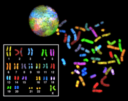
Multicolor FISH and the older spectral karyotyping are molecular cytogenetic techniques used to simultaneously visualize all the pairs of chromosomes in an organism in different colors. Fluorescently labeled probes for each chromosome are made by labeling chromosome-specific DNA with different fluorophores. Because there are a limited number of spectrally distinct fluorophores, a combinatorial labeling method is used to generate many different colors. Fluorophore combinations are captured and analyzed by a fluorescence microscope using up to 7 narrow-banded fluorescence filters or, in the case of spectral karyotyping, by using an interferometer attached to a fluorescence microscope. In the case of an mFISH image, every combination of fluorochromes from the resulting original images is replaced by a pseudo color in a dedicated image analysis software. Thus, chromosomes or chromosome sections can be visualized and identified, allowing for the analysis of chromosomal rearrangements.[62] In the case of spectral karyotyping, image processing software assigns a pseudo color to each spectrally different combination, allowing the visualization of the individually colored chromosomes.[63]

Multicolor FISH is used to identify structural chromosome aberrations in cancer cells and other disease conditions when Giemsa banding or other techniques are not accurate enough.
Digital karyotyping
Digital karyotyping is a technique used to quantify the DNA copy number on a genomic scale. Short sequences of DNA from specific loci all over the genome are isolated and enumerated.[64] This method is also known as virtual karyotyping.
Chromosome abnormalities
Chromosome abnormalities can be numerical, as in the presence of extra or missing chromosomes, or structural, as in derivative chromosome, translocations, inversions, large-scale deletions or duplications. Numerical abnormalities, also known as aneuploidy, often occur as a result of nondisjunction during meiosis in the formation of a gamete; trisomies, in which three copies of a chromosome are present instead of the usual two, are common numerical abnormalities. Structural abnormalities often arise from errors in homologous recombination. Both types of abnormalities can occur in gametes and therefore will be present in all cells of an affected person's body, or they can occur during mitosis and give rise to a genetic mosaic individual who has some normal and some abnormal cells.
Chromosomal abnormalities that lead to disease in humans include
- Turner syndrome results from a single X chromosome (45, X or 45, X0).
- Klinefelter syndrome, the most common male chromosomal disease, otherwise known as 47, XXY is caused by an extra X chromosome.
- Edwards syndrome is caused by trisomy (three copies) of chromosome 18.
- Down syndrome, a common chromosomal disease, is caused by trisomy of chromosome 21.
- Patau syndrome is caused by trisomy of chromosome 13.
- Trisomy 9, believed to be the 4th most common trisomy has many long lived affected individuals but only in a form other than a full trisomy, such as Trisomy 9p syndrome or Mosaic trisomy 9. They often function quite well, but tend to have trouble with speech.
- Also documented are trisomy 8, and trisomy 16, although they generally do not survive to birth.
Some disorders arise from loss of just a piece of one chromosome, including
- Cri du chat (cry of the cat), from a truncated short arm on chromosome 5. The name comes from the babies' distinctive cry, caused by abnormal formation of the larynx.
- 1p36 Deletion syndrome, from the loss of part of the short arm of chromosome 1.
- Angelman syndrome – 50% of cases have a segment of the long arm of chromosome 15 missing; a deletion of the maternal genes, example of imprinting disorder.
- Prader-Willi syndrome – 50% of cases have a segment of the long arm of chromosome 15 missing; a deletion of the paternal genes, example of imprinting disorder.
Chromosomal abnormalities can also occur in cancerous cells of an otherwise genetically normal individual; one well-documented example is the Philadelphia chromosome, a translocation mutation commonly associated with chronic myelogenous leukemia and less often with acute lymphoblastic leukemia.
See also
References
- ↑ Concise Oxford Dictionary
- 1 2 3 White 1973, p. 28
- ↑ Stebbins, G.L. (1950). "Chapter XII: The Karyotype". Variation and evolution in plants. Columbia University Press.
- ↑ King, R.C.; Stansfield, W.D.; Mulligan, P.K. (2006). A dictionary of genetics (7th ed.). Oxford University Press. p. 242.
- ↑ "Karyosystematics".
- ↑ Levitsky G.A. 1924. The material basis of heredity. State Publication Office of the Ukraine, Kiev. [in Russian]
- ↑ Levitsky G.A. (1931). "The morphology of chromosomes". Bull. Applied Bot. Genet. Plant Breed. 27: 19–174.
- ↑ Darlington C.D. 1939. Evolution of genetic systems. Cambridge University Press. 2nd ed, revised and enlarged, 1958. Oliver & Boyd, Edinburgh.
- 1 2 White M.J.D. 1973. Animal cytology and evolution. 3rd ed, Cambridge University Press.
- ↑ Kottler MJ (1974). "From 48 to 46: cytological technique, preconception, and the counting of human chromosomes". Bull Hist Med. 48 (4): 465–502. PMID 4618149.
- ↑ von Winiwarter H. (1912). "Études sur la spermatogenèse humaine". Archives de Biologie. 27 (93): 147–9.
- ↑ Painter T.S. (1922). "The spermatogenesis of man". Anat. Res. 23: 129.
- ↑ Painter T.S. (1923). "Studies in mammalian spermatogenesis II". J. Expt. Zoology. 37 (3): 291–336. doi:10.1002/jez.1400370303.
- ↑ Wright, Pearce (11 December 2001). "Joe Hin Tjio The man who cracked the chromosome count". The Guardian.
- ↑ Tjio J.H; Levan A. (1956). "The chromosome number of man". Hereditas. 42: 1–6. doi:10.1111/j.1601-5223.1956.tb03010.x.
- 1 2 Hsu T.C. 1979. Human and mammalian cytogenetics: a historical perspective. Springer-Verlag, NY.
- ↑ Human chromosome 2 is a fusion of two ancestral chromosomes Alec MacAndrew; accessed 18 May 2006.
- ↑ Evidence of common ancestry: human chromosome 2 (video) 2007
- ↑ A preparation which includes the dyes Methylene Blue, Eosin Y and Azure-A,B,C
- 1 2 Gustashaw K.M. 1991. Chromosome stains. In The ACT Cytogenetics Laboratory Manual 2nd ed, ed. M.J. Barch. The Association of Cytogenetic Technologists, Raven Press, New York.
- ↑ Stebbins, G.L. (1971). Chromosomal evolution in higher plants. London: Arnold. pp. 85–86.
- 1 2 Thompson & Thompson Genetics in Medicine 7th Ed
- ↑ Godfrey LR, Masters JC (August 2000). "Kinetochore reproduction theory may explain rapid chromosome evolution". Proc. Natl. Acad. Sci. U.S.A. 97 (18): 9821–3. Bibcode:2000PNAS...97.9821G. doi:10.1073/pnas.97.18.9821. PMC 34032
 . PMID 10963652.
 - ↑ Maynard Smith J. 1998. Evolutionary genetics. 2nd ed, Oxford. p218-9
- ↑ Goday C, Esteban MR (March 2001). "Chromosome elimination in sciarid flies". BioEssays. 23 (3): 242–50. doi:10.1002/1521-1878(200103)23:3<242::AID-BIES1034>3.0.CO;2-P. PMID 11223881.
- ↑ Müller F, Bernard V, Tobler H (February 1996). "Chromatin diminution in nematodes". BioEssays. 18 (2): 133–8. doi:10.1002/bies.950180209. PMID 8851046.
- ↑ Wyngaard GA, Gregory TR (December 2001). "Temporal control of DNA replication and the adaptive value of chromatin diminution in copepods". J. Exp. Zool. 291 (4): 310–6. doi:10.1002/jez.1131. PMID 11754011.
- ↑ Gilbert S.F. 2006. Developmental biology. Sinauer Associates, Stamford CT. 8th ed, Chapter 9
- ↑ King, Stansfield & Mulligan 2006
- ↑ Carrel L, Willard H (2005). "X-inactivation profile reveals extensive variability in X-linked gene expression in females". Nature. 434 (7031): 400–404. doi:10.1038/nature03479. PMID 15772666.
- ↑ Wurster DH, Benirschke K (June 1970). "Indian muntjac, Muntiacus muntjak: a deer with a low diploid chromosome number". Science. 168 (3937): 1364–6. Bibcode:1970Sci...168.1364W. doi:10.1126/science.168.3937.1364. PMID 5444269.
- ↑ Crosland M.W.J.; Crozier, R.H. (1986). "Myrmecia pilosula, an ant with only one pair of chromosomes". Science. 231 (4743): 1278. Bibcode:1986Sci...231.1278C. doi:10.1126/science.231.4743.1278. PMID 17839565.
- ↑ Khandelwal S. (1990). "Chromosome evolution in the genus Ophioglossum L". Botanical Journal of the Linnean Society. 102 (3): 205–217. doi:10.1111/j.1095-8339.1990.tb01876.x.
- ↑ Kim, D.S.; Nam, Y.K.; Noh, J.K.; Park, C.H.; Chapman, F.A. (2005). "Karyotype of North American shortnose sturgeon Acipenser brevirostrum with the highest chromosome number in the Acipenseriformes" (PDF). Ichthyological Research. 52 (1): 94–97. doi:10.1007/s10228-004-0257-z.
- ↑ Matthey, R. (1945-05-15). "L'evolution de la formule chromosomiale chez les vertébrés". Experientia (Basel). 1 (2): 50–56. doi:10.1007/BF02153623.
- ↑ de Oliveira, R.R.; Feldberg, E.; dos Anjos, M. B.; Zuanon, J. (July–September 2007). "Karyotype characterization and ZZ/ZW sex chromosome heteromorphism in two species of the catfish genus Ancistrus Kner, 1854 (Siluriformes: Loricariidae) from the Amazon basin". Neotropical Ichthyology. Sociedade Brasileira de Ictiologia. 5 (3): 301–6. doi:10.1590/S1679-62252007000300010.
- ↑ Pellicciari, C.; Formenti, D.; Redi, C.A.; Manfredi, M.G.; Romanini, (February 1982). "DNA content variability in primates". Journal of Human Evolution. 11 (2): 131–141. doi:10.1016/S0047-2484(82)80045-6.
- ↑ Souza, A.L.G.; de O. Corrêa, M.M.; de Aguilar, C.T.; Pessôa, L.M. (February 2011). "A new karyotype of Wiedomys pyrrhorhinus (Rodentia: Sigmodontinae) from Chapada Diamantina, northeastern Brazil" (PDF). Zoologia. 28 (1): 92–96. doi:10.1590/S1984-46702011000100013.
- ↑ Weksler, M.; Bonvicino, C.R. (2005-01-03). "Taxonomy of pygmy rice rats genus Oligoryzomys Bangs, 1900 (Rodentia, Sigmodontinae) of the Brazilian Cerrado, with the description of two new species" (PDF). Arquivos do Museu Nacional, Rio de Janeiro. 63 (1): 113–130. ISSN 0365-4508.
- ↑ Stebbins, G.L. (1940). "The significance of polyploidy in plant evolution". The American Naturalist. 74 (750): 54–66. doi:10.1086/280872.
- ↑ Stebbins 1950
- ↑ Comai L (November 2005). "The advantages and disadvantages of being polyploid". Nat. Rev. Genet. 6 (11): 836–46. doi:10.1038/nrg1711. PMID 16304599.
- ↑ Adams KL, Wendel JF (April 2005). "Polyploidy and genome evolution in plants". Curr. Opin. Plant Biol. 8 (2): 135–41. doi:10.1016/j.pbi.2005.01.001. PMID 15752992.
- ↑ Stebbins 1971
- ↑ Gregory, T.R.; Mable, B.K. (2011). "Ch. 8: Polyploidy in animals". In Gregory, T. Ryan. The Evolution of the Genome. Academic Press. pp. 427–517. ISBN 978-0-08-047052-8.
- ↑ White, M.J.D. (1973). The chromosomes (6th ed.). London: Chapman & Hall. p. 45.
- ↑ Lilly M.A.; Duronio R.J. (2005). "New insights into cell cycle control from the Drosophila endocycle". Oncogene. 24 (17): 2765–75. doi:10.1038/sj.onc.1208610. PMID 15838513.
- ↑ Edgar BA, Orr-Weaver TL (May 2001). "Endoreplication cell cycles: more for less". Cell. 105 (3): 297–306. doi:10.1016/S0092-8674(01)00334-8. PMID 11348589.
- ↑ Nagl W. 1978. Endopolyploidy and polyteny in differentiation and evolution: towards an understanding of quantitative and qualitative variation of nuclear DNA in ontogeny and phylogeny. Elsevier, New York.
- ↑ Stebbins, G. Ledley, Jr. 1972. Chromosomal evolution in higher plants. Nelson, London. p18
- ↑ IJdo JW, Baldini A, Ward DC, Reeders ST, Wells RA (October 1991). "Origin of human chromosome 2: an ancestral telomere-telomere fusion". Proc. Natl. Acad. Sci. U.S.A. 88 (20): 9051–5. Bibcode:1991PNAS...88.9051I. doi:10.1073/pnas.88.20.9051. PMC 52649. PMID 1924367.
- ↑ Rieger, R.; Michaelis, A.; Green, M.M. (1968). A glossary of genetics and cytogenetics: Classical and molecular. New York: Springer-Verlag. ISBN 9780387076683.
- ↑ White 1973, p. 169
- ↑ Clague, D.A.; Dalrymple, G.B. (1987). "The Hawaiian-Emperor volcanic chain, Part I. Geologic evolution". In Decker, R.W.; Wright, T.L.; Stauffer, P.H. Volcanism in Hawaii (PDF). 1. pp. 5–54. U.S. Geological Survey Professional Paper 1350.
- ↑ Carson HL (June 1970). "Chromosome tracers of the origin of species". Science. 168 (3938): 1414–8. Bibcode:1970Sci...168.1414C. doi:10.1126/science.168.3938.1414. PMID 5445927.
- ↑ Carson HL (March 1983). "Chromosomal sequences and interisland colonizations in Hawaiian Drosophila". Genetics. 103 (3): 465–82. PMC 1202034. PMID 17246115.
- ↑ Carson H.L. (1992). "Inversions in Hawaiian Drosophila". In Krimbas, C.B.; Powell, J.R. Drosophila inversion polymorphism. Boca Raton FL: CRC Press. pp. 407–439. ISBN 0849365473.
- ↑ Kaneshiro, K.Y.; Gillespie, R.G.; Carson, H.L. (1995). "Chromosomes and male genitalia of Hawaiian Drosophila: tools for interpreting phylogeny and geography". In Wagner, W.L.; Funk, E. Hawaiian biogeography: evolution on a hot spot archipelago. Washington DC: Smithsonian Institution Press. pp. 57–71.
- ↑ Craddock E.M. (2000). "Speciation processes in the adaptive radiation of Hawaiian plants and animals". Evolutionary Biology. 31: 1–43. doi:10.1007/978-1-4615-4185-1_1. ISBN 978-1-4613-6877-9.
- ↑ Ziegler, Alan C. (2002). Hawaiian natural history, ecology, and evolution. University of Hawaii Press. ISBN 978-0-8248-2190-6.
- ↑ Lisa G. Shaffer; Niels Tommerup, eds. (2005). ISCN 2005: An International System for Human Cytogenetic Nomenclature. Switzerland: S. Karger AG. ISBN 3-8055-8019-3.
- ↑ Liehr T, Starke H, Weise A, Lehrer H, Claussen U (January 2004). "Multicolour FISH probe sets and their applications". Histol Histopathol. 19 (1): 229–237. PMID 14702191.
- ↑ Schröck E, du Manoir S, Veldman T, et al. (July 1996). "Multicolor spectral karyotyping of human chromosomes". Science. 273 (5274): 494–7. Bibcode:1996Sci...273..494S. doi:10.1126/science.273.5274.494. PMID 8662537.
- ↑ Wang TL, Maierhofer C, Speicher MR, et al. (December 2002). "Digital karyotyping". Proc. Natl. Acad. Sci. U.S.A. 99 (25): 16156–61. Bibcode:2002PNAS...9916156W. doi:10.1073/pnas.202610899. PMC 138581. PMID 12461184.
External links
-
 Media related to Karyotypes at Wikimedia Commons
 - Making a karyotype, an online activity from the University of Utah's Genetic Science Learning Center.
- Karyotyping activity with case histories from the University of Arizona's Biology Project.
- Printable karyotype project from Biology Corner, a resource site for biology and science teachers.
- Chromosome Staining and Banding Techniques
- Bjorn Biosystems for Karyotyping and FISH
