Time dependent vector field

Part of a series of articles about

Definitions
Derivative (generalizations) Differential infinitesimal of a function total
Concepts
Differentiation notation Second derivative Third derivative Change of variables Implicit differentiation Related rates Taylor's theorem
Rules and identities
Sum Product Chain Power Quotient General Leibniz Faà di Bruno's formula

Integral

Definitions
Lists of integrals
Antiderivative Integral (improper) Riemann integral Lebesgue integration Contour integration
Integration by
Parts Discs Cylindrical shells Substitution (trigonometric) Partial fractions Order Reduction formulae

Series

Convergence tests
Geometric (arithmetico-geometric) Harmonic Alternating Power Binomial Taylor
Summand limit (term test) Ratio Root Integral Direct comparison Limit comparison Alternating series Cauchy condensation Dirichlet Abel

Vector

Theorems
Gradient Divergence Curl Laplacian Directional derivative Identities
Divergence Gradient Green's Kelvin–Stokes

Multivariable

Formalisms
Matrix Tensor Exterior Geometric
Definitions
Partial derivative Multiple integral Line integral Surface integral Volume integral Jacobian Hessian matrix

Specialized

In mathematics, a time dependent vector field is a construction in vector calculus which generalizes the concept of vector fields. It can be thought of as a vector field which moves as time passes. For every instant of time, it associates a vector to every point in a Euclidean space or in a manifold.

Definition

A time dependent vector field on a manifold M is a map from an open subset $\Omega \subset \Bbb{R} \times M$ on $TM$

X: \Omega \subset \Bbb{R} \times M \longrightarrow TM

(t,x) \longmapsto X(t,x)=X_t(x) \in T_xM

such that for every $(t,x) \in \Omega$ , $X_t(x)$ is an element of $T_xM$ .

For every $t \in \Bbb{R}$ such that the set

\Omega_t=\{x \in M | (t,x) \in \Omega \} \subset M

is nonempty, $X_t$ is a vector field in the usual sense defined on the open set $\Omega_t \subset M$ .

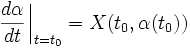
Associated differential equation

Given a time dependent vector field X on a manifold M, we can associate to it the following differential equation:

\frac{dx}{dt}=X(t,x)

which is called nonautonomous by definition.

Integral curve

An integral curve of the equation above (also called an integral curve of X) is a map

\alpha : I \subset \Bbb{R} \longrightarrow M

such that $\forall t_0 \in I$ , $(t_0,\alpha (t_0))$ is an element of the domain of definition of X and

\frac{d \alpha}{dt} \left.{\!\!\frac{}{}}\right|_{t=t_0} =X(t_0,\alpha (t_0))

Relationship with vector fields in the usual sense

A vector field in the usual sense can be thought of as a time dependent vector field defined on $\Bbb{R} \times M$ even though its value on a point $(t,x)$ does not depend on the component $t \in \Bbb{R}$ .

Conversely, given a time dependent vector field X defined on $\Omega \subset \Bbb{R} \times M$ , we can associate to it a vector field in the usual sense $\tilde{X}$ on $\Omega$ such that the autonomous differential equation associated to $\tilde{X}$ is essentially equivalent to the nonautonomous differential equation associated to X. It suffices to impose:

\tilde{X}(t,x)=(1,X(t,x))

for each $(t,x) \in \Omega$ , where we identify $T_{(t,x)}(\Bbb{R}\times M)$ with $\Bbb{R}\times T_x M$ . We can also write it as:

\tilde{X}=\frac{\partial{}}{\partial{t}}+X

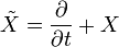To each integral curve of X, we can associate one integral curve of $\tilde{X}$ , and vice versa.

Flow

The flow of a time dependent vector field X, is the unique differentiable map

F:D(X) \subset \Bbb{R} \times \Omega \longrightarrow M

such that for every $(t_0,x) \in \Omega$ ,

t \longrightarrow F(t,t_0,x)

is the integral curve $\alpha$ of X that satisfies $\alpha (t_0) = x$ .

Properties

We define $F_{t,s}$ as $F_{t,s}(p)=F(t,s,p)$

If $(t_1,t_0,p) \in D(X)$ and $(t_2,t_1,F_{t_1,t_0}(p)) \in D(X)$ then $F_{t_2,t_1} \circ F_{t_1,t_0}(p)=F_{t_2,t_0}(p)$
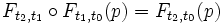
$\forall t,s$ , $F_{t,s}$ is a diffeomorphism with inverse $F_{s,t}$ .

Applications

Let X and Y be smooth time dependent vector fields and $F$ the flow of X. The following identity can be proved:

\frac{d}{dt} \left .{\!\!\frac{}{}}\right|_{t=t_1} (F^*_{t,t_0} Y_t)_p = \left( F^*_{t_1,t_0} \left( [X_{t_1},Y_{t_1}] + \frac{d}{dt} \left .{\!\!\frac{}{}}\right|_{t=t_1} Y_t \right) \right)_p

Also, we can define time dependent tensor fields in an analogous way, and prove this similar identity, assuming that $\eta$ is a smooth time dependent tensor field:

\frac{d}{dt} \left .{\!\!\frac{}{}}\right|_{t=t_1} (F^*_{t,t_0} \eta_t)_p = \left( F^*_{t_1,t_0} \left( \mathcal{L}_{X_{t_1}}\eta_{t_1} + \frac{d}{dt} \left .{\!\!\frac{}{}}\right|_{t=t_1} \eta_t \right) \right)_p

This last identity is useful to prove the Darboux theorem.

References

Lee, John M., Introduction to Smooth Manifolds, Springer-Verlag, New York (2003) ISBN 0-387-95495-3. Graduate-level textbook on smooth manifolds.

This article is issued from Wikipedia - version of the 7/4/2015. The text is available under the Creative Commons Attribution/Share Alike but additional terms may apply for the media files.