Gini coefficient
The Gini coefficient (sometimes expressed as a Gini ratio or a normalized Gini index) (/dʒini/ jee-nee) is a measure of statistical dispersion intended to represent the income distribution of a nation's residents, and is the most commonly used measure of inequality. It was developed by the Italian statistician and sociologist Corrado Gini and published in his 1912 paper Variability and Mutability (Italian: Variabilità e mutabilità).[1][2]
The Gini coefficient measures the inequality among values of a frequency distribution (for example, levels of income). A Gini coefficient of zero expresses perfect equality, where all values are the same (for example, where everyone has the same income). A Gini coefficient of 1 (or 100%) expresses maximal inequality among values (e.g., for a large number of people, where only one person has all the income or consumption, and all others have none, the Gini coefficient will be very nearly one).[3][4] However, a value greater than one may occur if some persons represent negative contribution to the total (for example, having negative income or wealth). For larger groups, values close to or above 1 are very unlikely in practice. Given the normalization of both the cumulative population and the cumulative share of income used to calculate the Gini coefficient, the measure is not overly sensitive to the specifics of the income distribution, but rather only on how incomes vary relative to the other members of a population. The exception to this is in the redistribution of wealth resulting in a minimum income for all people. When the population is sorted, if their income distribution were to approximate a well known function, then some representative values could be calculated.
The Gini coefficient was proposed by Gini as a measure of inequality of income or wealth.[5] For OECD countries, in the late 20th century, considering the effect of taxes and transfer payments, the income Gini coefficient ranged between 0.24 and 0.49, with Slovenia the lowest and Chile the highest.[6] African countries had the highest pre-tax Gini coefficients in 2008–2009, with South Africa the world's highest, variously estimated to be 0.63 to 0.7,[7][8] although this figure drops to 0.52 after social assistance is taken into account, and drops again to 0.47 after taxation.[9] The global income Gini coefficient in 2005 has been estimated to be between 0.61 and 0.68 by various sources.[10][11]
There are some issues in interpreting a Gini coefficient. The same value may result from many different distribution curves. The demographic structure should be taken into account. Countries with an aging population, or with a baby boom, experience an increasing pre-tax Gini coefficient even if real income distribution for working adults remains constant. Scholars have devised over a dozen variants of the Gini coefficient.[12][13][14]
Definition

The graph shows that the Gini coefficient is equal to the area marked A divided by the sum of the areas marked A and B, that is, Gini = A / (A + B). It is also equal to 2A and to 1 - 2B due to the fact that A + B = 0.5 (since the axes scale from 0 to 1).
The Gini coefficient is usually defined mathematically based on the Lorenz curve, which plots the proportion of the total income of the population (y axis) that is cumulatively earned by the bottom x% of the population (see diagram). The line at 45 degrees thus represents perfect equality of incomes. The Gini coefficient can then be thought of as the ratio of the area that lies between the line of equality and the Lorenz curve (marked A in the diagram) over the total area under the line of equality (marked A and B in the diagram); i.e., G = A / (A + B). It is also equal to 2A and to 1 - 2B due to the fact that A + B = 0.5 (since the axes scale from 0 to 1).
If all people have non-negative income (or wealth, as the case may be), the Gini coefficient can theoretically range from 0 (complete equality) to 1 (complete inequality); it is sometimes expressed as a percentage ranging between 0 and 100. In practice, both extreme values are not quite reached. If negative values are possible (such as the negative wealth of people with debts), then the Gini coefficient could theoretically be more than 1. Normally the mean (or total) is assumed positive, which rules out a Gini coefficient less than zero.
An alternative approach would be to consider the Gini coefficient as half of the relative mean absolute difference, which is a mathematical equivalence.[15] The mean absolute difference is the average absolute difference of all pairs of items of the population, and the relative mean absolute difference is the mean absolute difference divided by the average, to normalize for scale. if xi is the wealth or income of person i, and there are n persons, then the Gini coefficient G is given by:

When the income (or wealth) distribution is given as a continuous probability distribution function p(x), where p(x)dx is the fraction of the population with income x to x+dx, then the Gini coefficient is again half of the relative mean absolute difference:

where μ is the mean of the distribution and the lower limits of integration may be replaced by zero when all incomes are positive.

Calculation
Example: two levels of income

The most equal society will be one in which every person receives the same income (G = 0); the most unequal society will be one in which a single person receives 100% of the total income and the remaining people receive none (G = 1−1/N).
While the income distribution of any particular country need not follow simple functions, these functions give a qualitative understanding of the income distribution in a nation given the Gini coefficient. The effects of minimum income policy due to redistribution can be seen in the linear relationships.
An informative simplified case just distinguishes two levels of income, low and high. If the high income group is u % of the population and earns a fraction f % of all income, then the Gini coefficient is f − u. An actual more graded distribution with these same values u and f will always have a higher Gini coefficient than f − u.
The proverbial case where the richest 20% have 80% of all income would lead to an income Gini coefficient of at least 60%.
An often cited case that 1% of all the world's population owns 50% of all wealth, means a wealth Gini coefficient of at least 49%.
Alternate expressions
In some cases, this equation can be applied to calculate the Gini coefficient without direct reference to the Lorenz curve. For example, (taking y to mean the income or wealth of a person or household):
- For a population uniform on the values yi, i = 1 to n, indexed in non-decreasing order (yi ≤ yi+1):
- This may be simplified to:
- This formula actually applies to any real population, since each person can be assigned his or her own yi.[16]


Since the Gini coefficient is half the relative mean absolute difference, it can also be calculated using formulas for the relative mean absolute difference. For a random sample S consisting of values yi, i = 1 to n, that are indexed in non-decreasing order (yi ≤ yi+1), the statistic:

- is a consistent estimator of the population Gini coefficient, but is not, in general, unbiased. Like G, G (S) has a simpler form:
- .

There does not exist a sample statistic that is in general an unbiased estimator of the population Gini coefficient, like the relative mean absolute difference.
Discrete probability distribution
For a discrete probability distribution with probability mass function f ( yi ), i = 1 to n, where f ( yi ) is the fraction of the population with income or wealth yi >0, the Gini coefficient is:
- where


- If the points with nonzero probabilities are indexed in increasing order (yi < yi+1) then:
- where
- and . These formulae are also applicable in the limit as .


Continuous probability distribution
When the population is large, the income distribution may be represented by a continuous probability density function f(x) where f(x) dx is the fraction of the population with wealth or income in the interval dx about x. If F(x) is the cumulative distribution function for f(x), then the Lorenz curve L(F) may then be represented as a function parametric in L(x) and F(x) and the value of B can be found by integration:

The Gini coefficient can also be calculated directly from the cumulative distribution function of the distribution F(y). Defining μ as the mean of the distribution, and specifying that F(y) is zero for all negative values, the Gini coefficient is given by:

The latter result comes from integration by parts. (Note that this formula can be applied when there are negative values if the integration is taken from minus infinity to plus infinity.)
The Gini coefficient may be expressed in terms of the quantile function Q(F) (inverse of the cumulative distribution function: Q(F(x))=x)

For some functional forms, the Gini index can be calculated explicitly. For example, if y follows a lognormal distribution with the standard deviation of logs equal to , then where is the error function ( since , where is the cumulative standard normal distribution).[17] In the table below, some examples are shown. The Dirac delta distribution represents the case where everyone has the same wealth (or income); it implies that there are no variations at all between incomes.


Income Distribution function PDF(x) Gini Coefficient Dirac delta function 0 Uniform distribution Exponential distribution Log-normal distribution Pareto distribution Chi-squared distribution Gamma distribution Weibull distribution Beta distribution


Other approaches
Sometimes the entire Lorenz curve is not known, and only values at certain intervals are given. In that case, the Gini coefficient can be approximated by using various techniques for interpolating the missing values of the Lorenz curve. If (Xk, Yk) are the known points on the Lorenz curve, with the Xk indexed in increasing order (Xk – 1 < Xk), so that:
- Xk is the cumulated proportion of the population variable, for k = 0,...,n, with X0 = 0, Xn = 1.
- Yk is the cumulated proportion of the income variable, for k = 0,...,n, with Y0 = 0, Yn = 1.
- Yk should be indexed in non-decreasing order (Yk > Yk – 1)
If the Lorenz curve is approximated on each interval as a line between consecutive points, then the area B can be approximated with trapezoids and:

is the resulting approximation for G. More accurate results can be obtained using other methods to approximate the area B, such as approximating the Lorenz curve with a quadratic function across pairs of intervals, or building an appropriately smooth approximation to the underlying distribution function that matches the known data. If the population mean and boundary values for each interval are also known, these can also often be used to improve the accuracy of the approximation.
The Gini coefficient calculated from a sample is a statistic and its standard error, or confidence intervals for the population Gini coefficient, should be reported. These can be calculated using bootstrap techniques but those proposed have been mathematically complicated and computationally onerous even in an era of fast computers. Ogwang (2000) made the process more efficient by setting up a "trick regression model" in which respective income variables in the sample are ranked with the lowest income being allocated rank 1. The model then expresses the rank (dependent variable) as the sum of a constant A and a normal error term whose variance is inversely proportional to yk;

Ogwang showed that G can be expressed as a function of the weighted least squares estimate of the constant A and that this can be used to speed up the calculation of the jackknife estimate for the standard error. Giles (2004) argued that the standard error of the estimate of A can be used to derive that of the estimate of G directly without using a jackknife at all. This method only requires the use of ordinary least squares regression after ordering the sample data. The results compare favorably with the estimates from the jackknife with agreement improving with increasing sample size.[18]
However it has since been argued that this is dependent on the model's assumptions about the error distributions (Ogwang 2004) and the independence of error terms (Reza & Gastwirth 2006) and that these assumptions are often not valid for real data sets. It may therefore be better to stick with jackknife methods such as those proposed by Yitzhaki (1991) and Karagiannis and Kovacevic (2000). The debate continues.
Guillermina Jasso[19] and Angus Deaton[20] independently proposed the following formula for the Gini coefficient:

where is mean income of the population, Pi is the income rank P of person i, with income X, such that the richest person receives a rank of 1 and the poorest a rank of N. This effectively gives higher weight to poorer people in the income distribution, which allows the Gini to meet the Transfer Principle. Note that the Jasso-Deaton formula rescales the coefficient so that its value is 1 if all the are zero except one. Note however Allison's reply on the need to divide by N² instead.[21]


FAO explains another version of the formula.[22]
Generalized inequality indices
The Gini coefficient and other standard inequality indices reduce to a common form. Perfect equality—the absence of inequality—exists when and only when the inequality ratio, , equals 1 for all j units in some population (for example, there is perfect income equality when everyone's income equals the mean income , so that for everyone). Measures of inequality, then, are measures of the average deviations of the from 1; the greater the average deviation, the greater the inequality. Based on these observations the inequality indices have this common form:[23]


where pj weights the units by their population share, and f(rj) is a function of the deviation of each unit's rj from 1, the point of equality. The insight of this generalised inequality index is that inequality indices differ because they employ different functions of the distance of the inequality ratios (the rj) from 1.
Gini coefficients of income distributions
Gini coefficients of income are calculated on market income as well as disposable income basis. The Gini coefficient on market income—sometimes referred to as a pre-tax Gini coefficient—is calculated on income before taxes and transfers, and it measures inequality in income without considering the effect of taxes and social spending already in place in a country. The Gini coefficient on disposable income—sometimes referred to as after-tax Gini coefficient—is calculated on income after taxes and transfers, and it measures inequality in income after considering the effect of taxes and social spending already in place in a country.[6][24][25]
The difference in Gini indices between OECD countries, on after-taxes and transfers basis, is significantly narrower.[25] For OECD countries, over 2008–2009 period, Gini coefficient on pre-taxes and transfers basis for total population ranged between 0.34 and 0.53, with South Korea the lowest and Italy the highest. Gini coefficient on after-taxes and transfers basis for total population ranged between 0.25 and 0.48, with Denmark the lowest and Mexico the highest. For United States, the country with the largest population in OECD countries, the pre-tax Gini index was 0.49, and after-tax Gini index was 0.38, in 2008–2009. The OECD averages for total population in OECD countries was 0.46 for pre-tax income Gini index and 0.31 for after-tax income Gini Index.[6][26] Taxes and social spending that were in place in 2008–2009 period in OECD countries significantly lowered effective income inequality, and in general, "European countries—especially Nordic and Continental welfare states—achieve lower levels of income inequality than other countries."[27]
Using the Gini can help quantify differences in welfare and compensation policies and philosophies. However it should be borne in mind that the Gini coefficient can be misleading when used to make political comparisons between large and small countries or those with different immigration policies (see limitations of Gini coefficient section).
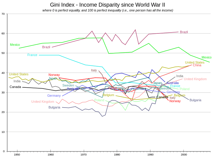
The Gini coefficient for the entire world has been estimated by various parties to be between 0.61 and 0.68.[10][11][28] The graph shows the values expressed as a percentage in their historical development for a number of countries.
Regional income Gini indices
According to UNICEF, Latin America and the Caribbean region had the highest net income Gini index in the world at 48.3, on unweighted average basis in 2008. The remaining regional averages were: sub-Saharan Africa (44.2), Asia (40.4), Middle East and North Africa (39.2), Eastern Europe and Central Asia (35.4), and High-income Countries (30.9). Using the same method, the United States is claimed to have a Gini index of 36, while South Africa had the highest income Gini index score of 67.8.[29]
World income Gini index since 1800s
The table below presents the estimated world income Gini coefficients over the last 200 years, as calculated by Milanovic.[31] Taking income distribution of all human beings, the worldwide income inequality has been constantly increasing since the early 19th century. There was a steady increase in global income inequality Gini score from 1820 to 2002, with a significant increase between 1980 and 2002. This trend appears to have peaked and begun a reversal with rapid economic growth in emerging economies, particularly in the large populations of BRIC countries.[32]
| Year | World Gini coefficients[10][29][33] |
|---|---|
| 1820 | 0.43 |
| 1850 | 0.53 |
| 1870 | 0.56 |
| 1913 | 0.61 |
| 1929 | 0.62 |
| 1950 | 0.64 |
| 1960 | 0.64 |
| 1980 | 0.66 |
| 2002 | 0.71 |
| 2005 | 0.68 |
Gini coefficients of social development
Gini coefficient is widely used in fields as diverse as sociology, economics, health science, ecology, engineering and agriculture.[34] For example, in social sciences and economics, in addition to income Gini coefficients, scholars have published education Gini coefficients and opportunity Gini coefficients.
Gini coefficient of education
Education Gini index estimates the inequality in education for a given population.[35] It is used to discern trends in social development through educational attainment over time. From a study of 85 countries, Thomas, et al. estimate Mali had the highest education Gini index of 0.92 in 1990 (implying very high inequality in education attainment across the population), while the United States had the lowest education inequality Gini index of 0.14. Between 1960 and 1990, South Korea, China and India had the fastest drop in education inequality Gini Index. They also claim education Gini index for the United States slightly increased over the 1980–1990 period.
Gini coefficient of opportunity
Similar in concept to income Gini coefficient, opportunity Gini coefficient measures inequality of opportunity.[36][37][38] The concept builds on Amartya Sen's suggestion[39] that inequality coefficients of social development should be premised on the process of enlarging people's choices and enhancing their capabilities, rather than on the process of reducing income inequality. Kovacevic in a review of opportunity Gini coefficient explains that the coefficient estimates how well a society enables its citizens to achieve success in life where the success is based on a person's choices, efforts and talents, not his background defined by a set of predetermined circumstances at birth, such as, gender, race, place of birth, parent's income and circumstances beyond the control of that individual.
In 2003, Roemer[36][40] reported Italy and Spain exhibited the largest opportunity inequality Gini index amongst advanced economies.
Gini coefficients and income mobility
In 1978, Anthony Shorrocks introduced a measure based on income Gini coefficients to estimate income mobility.[41] This measure, generalized by Maasoumi and Zandvakili,[42] is now generally referred to as Shorrocks index, sometimes as Shorrocks mobility index or Shorrocks rigidity index. It attempts to estimate whether the income inequality Gini coefficient is permanent or temporary, and to what extent a country or region enables economic mobility to its people so that they can move from one (e.g. bottom 20%) income quantile to another (e.g. middle 20%) over time. In other words, Shorrocks index compares inequality of short-term earnings such as annual income of households, to inequality of long-term earnings such as 5-year or 10-year total income for same households.
Shorrocks index is calculated in number of different ways, a common approach being from the ratio of income Gini coefficients between short-term and long-term for the same region or country.[43]
A 2010 study using social security income data for the United States since 1937 and Gini-based Shorrocks indices concludes that income mobility in the United States has had a complicated history, primarily due to mass influx of women into the American labor force after World War II. Income inequality and income mobility trends have been different for men and women workers between 1937 and the 2000s. When men and women are considered together, the Gini coefficient-based Shorrocks index trends imply long-term income inequality has been substantially reduced among all workers, in recent decades for the United States.[43] Other scholars, using just 1990s data or other short periods have come to different conclusions.[44] For example, Sastre and Ayala, conclude from their study of income Gini coefficient data between 1993 and 1998 for six developed economies, that France had the least income mobility, Italy the highest, and the United States and Germany intermediate levels of income mobility over those 5 years.[45]
Features of Gini coefficient
The Gini coefficient has features that make it useful as a measure of dispersion in a population, and inequalities in particular.[22] It is a ratio analysis method making it easier to interpret. It also avoids references to a statistical average or position unrepresentative of most of the population, such as per capita income or gross domestic product. For a given time interval, Gini coefficient can therefore be used to compare diverse countries and different regions or groups within a country; for example states, counties, urban versus rural areas, gender and ethnic groups. Gini coefficients can be used to compare income distribution over time, thus it is possible to see if inequality is increasing or decreasing independent of absolute incomes.
Other useful features of the Gini coefficient include:[46] [47]
- Anonymity: it does not matter who the high and low earners are.
- Scale independence: the Gini coefficient does not consider the size of the economy, the way it is measured, or whether it is a rich or poor country on average.
- Population independence: it does not matter how large the population of the country is.
- Transfer principle: if income (less than the difference), is transferred from a rich person to a poor person the resulting distribution is more equal.
Countries by Gini Index
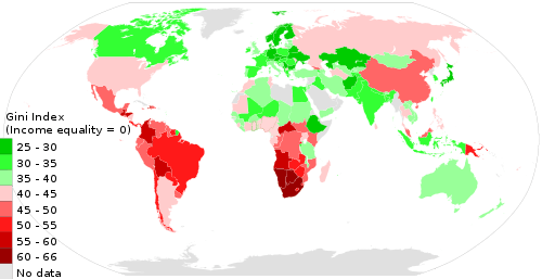
red = high, green = low inequality
A Gini index value above 50 is considered high; countries like the Seychelles, Brazil, Chile, Botswana and Central American countries can be found in this category. A Gini index value of 30 or above is considered medium; countries like Vietnam, Mexico, Poland, USA, Russia, and Venezuela can be found in this category. A Gini index value lower than 30 is considered low; countries like Austria, Afghanistan,India and Denmark can be found in this category.[48]
Limitations of Gini coefficient
The Gini coefficient is a relative measure. Its proper use and interpretation is controversial.[49] It is possible for the Gini coefficient of a developing country to rise (due to increasing inequality of income) while the number of people in absolute poverty decreases.[50] This is because the Gini coefficient measures relative, not absolute, wealth. Changing income inequality, measured by Gini coefficients, can be due to structural changes in a society such as growing population (baby booms, aging populations, increased divorce rates, extended family households splitting into nuclear families, emigration, immigration) and income mobility.[51] Gini coefficients are simple, and this simplicity can lead to oversights and can confuse the comparison of different populations; for example, while both Bangladesh (per capita income of $1,693) and the Netherlands (per capita income of $42,183) had an income Gini coefficient of 0.31 in 2010,[52] the quality of life, economic opportunity and absolute income in these countries are very different, i.e. countries may have identical Gini coefficients, but differ greatly in wealth. Basic necessities may be available to all in a developed economy, while in an undeveloped economy with the same Gini coefficient, basic necessities may be unavailable to most or unequally available, due to lower absolute wealth.
| Household Group | Country A Annual Income ($) | Country B Annual Income ($) |
|---|---|---|
| 1 | 20,000 | 9,000 |
| 2 | 30,000 | 40,000 |
| 3 | 40,000 | 48,000 |
| 4 | 50,000 | 48,000 |
| 5 | 60,000 | 55,000 |
| Total Income | $200,000 | $200,000 |
| Country's Gini | 0.2 | 0.2 |
- Different income distributions with the same Gini coefficient
Even when the total income of a population is the same, in certain situations two countries with different income distributions can have the same Gini index (e.g. cases when income Lorenz Curves cross).[22] Table A illustrates one such situation. Both countries have a Gini coefficient of 0.2, but the average income distributions for household groups are different. As another example, in a population where the lowest 50% of individuals have no income and the other 50% have equal income, the Gini coefficient is 0.5; whereas for another population where the lowest 75% of people have 25% of income and the top 25% have 75% of the income, the Gini index is also 0.5. Economies with similar incomes and Gini coefficients can have very different income distributions. Bellù and Liberati claim that to rank income inequality between two different populations based on their Gini indices is sometimes not possible, or misleading.[53]
- Extreme wealth inequality, yet low income Gini coefficient
A Gini index does not contain information about absolute national or personal incomes. Populations can have very low income Gini indices, yet simultaneously very high wealth Gini index. By measuring inequality in income, the Gini ignores the differential efficiency of use of household income. By ignoring wealth (except as it contributes to income) the Gini can create the appearance of inequality when the people compared are at different stages in their life. Wealthy countries such as Sweden can show a low Gini coefficient for disposable income of 0.31 thereby appearing equal, yet have very high Gini coefficient for wealth of 0.79 to 0.86 thereby suggesting an extremely unequal wealth distribution in its society.[54][55] These factors are not assessed in income-based Gini.
| Household number | Country A Annual Income ($) | Household combined number | Country A combined Annual Income ($) |
|---|---|---|---|
| 1 | 20,000 | 1 & 2 | 50,000 |
| 2 | 30,000 | ||
| 3 | 40,000 | 3 & 4 | 90,000 |
| 4 | 50,000 | ||
| 5 | 60,000 | 5 & 6 | 130,000 |
| 6 | 70,000 | ||
| 7 | 80,000 | 7 & 8 | 170,000 |
| 8 | 90,000 | ||
| 9 | 120,000 | 9 & 10 | 270,000 |
| 10 | 150,000 | ||
| Total Income | $710,000 | $710,000 | |
| Country's Gini | 0.303 | 0.293 |
- Small sample bias – sparsely populated regions more likely to have low Gini coefficient
Gini index has a downward-bias for small populations.[56] Counties or states or countries with small populations and less diverse economies will tend to report small Gini coefficients. For economically diverse large population groups, a much higher coefficient is expected than for each of its regions. Taking world economy as one, and income distribution for all human beings, for example, different scholars estimate global Gini index to range between 0.61 and 0.68.[10][11] As with other inequality coefficients, the Gini coefficient is influenced by the granularity of the measurements. For example, five 20% quantiles (low granularity) will usually yield a lower Gini coefficient than twenty 5% quantiles (high granularity) for the same distribution. Philippe Monfort has shown that using inconsistent or unspecified granularity limits the usefulness of Gini coefficient measurements.[57]
The Gini coefficient measure gives different results when applied to individuals instead of households, for the same economy and same income distributions. If household data is used, the measured value of income Gini depends on how the household is defined. When different populations are not measured with consistent definitions, comparison is not meaningful.
Deininger and Squire (1996) show that income Gini coefficient based on individual income, rather than household income, are different. For United States, for example, they find that individual income-based Gini coefficient was 0.35, while for France they report individual income-based Gini index to be 0.43. According to their individual focused method, in the 108 countries they studied, South Africa had the world's highest Gini coefficient at 0.62, Malaysia had Asia's highest Gini coefficient at 0.5, Brazil the highest at 0.57 in Latin America and Caribbean region, and Turkey the highest at 0.5 in OECD countries.[58]
| Income bracket (in 2010 adjusted dollars) | % of Population 1979 | % of Population 2010 |
|---|---|---|
| Under $15,000 | 14.6% | 13.7% |
| $15,000 – $24,999 | 11.9% | 12.0% |
| $25,000 – $34,999 | 12.1% | 10.9% |
| $35,000 – $49,999 | 15.4% | 13.9% |
| $50,000 – $74,999 | 22.1% | 17.7% |
| $75,000 – $99,999 | 12.4% | 11.4% |
| $100,000 – $149,999 | 8.3% | 12.1% |
| $150,000 – $199,999 | 2.0% | 4.5% |
| $200,000 and over | 1.2% | 3.9% |
| Total Households | 80,776,000 | 118,682,000 |
| United States' Gini on pre-tax basis | 0.404 | 0.469 |
- Gini coefficient is unable to discern the effects of structural changes in populations[51]
Expanding on the importance of life-span measures, the Gini coefficient as a point-estimate of equality at a certain time, ignores life-span changes in income. Typically, increases in the proportion of young or old members of a society will drive apparent changes in equality, simply because people generally have lower incomes and wealth when they are young than when they are old. Because of this, factors such as age distribution within a population and mobility within income classes can create the appearance of inequality when none exist taking into account demographic effects. Thus a given economy may have a higher Gini coefficient at any one point in time compared to another, while the Gini coefficient calculated over individuals' lifetime income is actually lower than the apparently more equal (at a given point in time) economy's.[14] Essentially, what matters is not just inequality in any particular year, but the composition of the distribution over time.
Kwok claims income Gini coefficient for Hong Kong has been high (0.434 in 2010[52]), in part because of structural changes in its population. Over recent decades, Hong Kong has witnessed increasing numbers of small households, elderly households and elderly living alone. The combined income is now split into more households. Many old people are living separately from their children in Hong Kong. These social changes have caused substantial changes in household income distribution. Income Gini coefficient, claims Kwok, does not discern these structural changes in its society.[51] Household money income distribution for the United States, summarized in Table C of this section, confirms that this issue is not limited to just Hong Kong. According to the US Census Bureau, between 1979 and 2010, the population of United States experienced structural changes in overall households, the income for all income brackets increased in inflation-adjusted terms, household income distributions shifted into higher income brackets over time, while the income Gini coefficient increased.[59][60]
Another limitation of Gini coefficient is that it is not a proper measure of egalitarianism, as it is only measures income dispersion. For example, if two equally egalitarian countries pursue different immigration policies, the country accepting a higher proportion of low-income or impoverished migrants will report a higher Gini coefficient and therefore may appear to exhibit more income inequality.
- Inability to value benefits and income from informal economy affects Gini coefficient accuracy
Some countries distribute benefits that are difficult to value. Countries that provide subsidized housing, medical care, education or other such services are difficult to value objectively, as it depends on quality and extent of the benefit. In absence of free markets, valuing these income transfers as household income is subjective. The theoretical model of Gini coefficient is limited to accepting correct or incorrect subjective assumptions.
In subsistence-driven and informal economies, people may have significant income in other forms than money, for example through subsistence farming or bartering. These income tend to accrue to the segment of population that is below-poverty line or very poor, in emerging and transitional economy countries such as those in sub-Saharan Africa, Latin America, Asia and Eastern Europe. Informal economy accounts for over half of global employment and as much as 90 per cent of employment in some of the poorer sub-Saharan countries with high official Gini inequality coefficients. Schneider et al., in their 2010 study of 162 countries,[61] report about 31.2%, or about $20 trillion, of world's GDP is informal. In developing countries, the informal economy predominates for all income brackets except for the richer, urban upper income bracket populations. Even in developed economies, between 8% (United States) to 27% (Italy) of each nation's GDP is informal, and resulting informal income predominates as a livelihood activity for those in the lowest income brackets.[62] The value and distribution of the incomes from informal or underground economy is difficult to quantify, making true income Gini coefficients estimates difficult.[63][64] Different assumptions and quantifications of these incomes will yield different Gini coefficients.[65][66][67]
Gini has some mathematical limitations as well. It is not additive and different sets of people cannot be averaged to obtain the Gini coefficient of all the people in the sets.
Alternatives to Gini coefficient
Given the limitations of Gini coefficient, other statistical methods are used in combination or as an alternative measure of population dispersity. For example, entropy measures are frequently used (e.g. the Theil Index, the Atkinson index and the generalized entropy index). These measures attempt to compare the distribution of resources by intelligent agents in the market with a maximum entropy random distribution, which would occur if these agents acted like non-intelligent particles in a closed system following the laws of statistical physics.
Relation to other statistical measures
The Gini coefficient closely related to the AUC (Area Under receiver operating characteristic Curve) measure of performance.[68] The relation follows the formula Gini coefficient is also closely related to Mann–Whitney U.

The Gini index is also related to Pietra index—both of which are a measure of statistical heterogeneity and are derived from Lorenz curve and the diagonal line.[69][70]
In certain fields such as ecology, Simpson's index is used, which is related to Gini. Simpson index scales as mirror opposite to Gini; that is, with increasing diversity Simpson index takes a smaller value (0 means maximum, 1 means minimum heterogeneity per classic Simpson index). Simpson index is sometimes transformed by subtracting the observed value from the maximum possible value of 1, and then it is known as Gini-Simpson Index.[71]
Other uses
Although the Gini coefficient is most popular in economics, it can in theory be applied in any field of science that studies a distribution. For example, in ecology the Gini coefficient has been used as a measure of biodiversity, where the cumulative proportion of species is plotted against cumulative proportion of individuals.[72] In health, it has been used as a measure of the inequality of health related quality of life in a population.[73] In education, it has been used as a measure of the inequality of universities.[74] In chemistry it has been used to express the selectivity of protein kinase inhibitors against a panel of kinases.[75] In engineering, it has been used to evaluate the fairness achieved by Internet routers in scheduling packet transmissions from different flows of traffic.[76]
The Gini coefficient is sometimes used for the measurement of the discriminatory power of rating systems in credit risk management.[77]
A 2005 study accessed US census data to measure home computer ownership and used the Gini coefficient to measure inequalities amongst whites and African Americans. Results indicated that although decreasing overall, home computer ownership inequality is substantially smaller among white households. [78]
A 2016 peer-reviewed study titled Employing the Gini coefficient to measure participation inequality in treatment-focused Digital Health Social Networks [79] illustrated that the Gini coefficient was helpful and accurate in measuring shifts in inequality, however as a standalone metric it failed to incorporate overall network size.
The discriminatory power refers to a credit risk model's ability to differentiate between defaulting and non-defaulting clients. The formula , in calculation section above, may be used for the final model and also at individual model factor level, to quantify the discriminatory power of individual factors. It is related to accuracy ratio in population assessment models.

See also
- Diversity index
- Economic inequality
- Great Gatsby curve
- Human Poverty Index
- Kuznets curve
- Pareto distribution
- Hoover index (a.k.a. Robin Hood index)
- ROC analysis
- Social welfare provision
- Suits index
- Utopia
- Welfare economics
- List of countries by distribution of wealth
- List of countries by income equality
- List of U.S. states by income equality
- Herfindahl index
References
- ↑ Gini (1912).
- ↑ Gini, C. (1909). "Concentration and dependency ratios" (in Italian). English translation in Rivista di Politica Economica, 87 (1997), 769–789.
- ↑ "Current Population Survey (CPS) – Definitions and Explanations". US Census Bureau.
- ↑ Note: Gini coefficient becomes 1, only in a large population where one person has all the income. In the special case of just two people, where one has no income and the other has all the income, the Gini coefficient is 0.5. For 5 people set, where 4 have no income and the fifth has all the income, the Gini coefficient is 0.8. See: FAO, United Nations – Inequality Analysis, The Gini Index Module (PDF format), fao.org.
- ↑ Gini, C. (1936). "On the Measure of Concentration with Special Reference to Income and Statistics", Colorado College Publication, General Series No. 208, 73–79.
- 1 2 3 "Income distribution – Inequality: Income distribution – Inequality – Country tables". OECD. 2012. Archived from the original on 9 November 2014.
- ↑ "South Africa Snapshot, Q4 2013" (PDF). KPMG. 2013.
- ↑ "Gini Coefficient". United Nations Development Program. 2012.
- ↑ Schüssler, Mike (16 July 2014). "The Gini is still in the bottle". Money Web. Retrieved 24 November 2014.
- 1 2 3 4 Hillebrand, Evan (June 2009). "Poverty, Growth, and Inequality over the Next 50 Years" (PDF). FAO, United Nations – Economic and Social Development Department.
- 1 2 3 "The Real Wealth of Nations: Pathways to Human Development, 2010" (PDF). United Nations Development Program. 2011. pp. 72–74. ISBN 978-0-230-28445-6.
- ↑ Yitzhaki, Shlomo (1998). "More than a Dozen Alternative Ways of Spelling Gini" (PDF). Economic Inequality. 8: 13–30.
- ↑ Sung, Myung Jae (August 2010). "Population Aging, Mobility of Quarterly Incomes, and Annual Income Inequality: Theoretical Discussion and Empirical Findings".
- 1 2 Blomquist, N. (1981). "A comparison of distributions of annual and lifetime income: Sweden around 1970". Review of Income and Wealth. 27 (3): 243–264. doi:10.1111/j.1475-4991.1981.tb00227.x.
- ↑ Sen, Amartya (1977), On Economic Inequality (2nd ed.), Oxford: Oxford University Press
- ↑ "Gini Coefficient". Wolfram Mathworld.
- ↑ Crow, E. L., & Shimizu, K. (Eds.). (1988). Lognormal distributions: Theory and applications (Vol. 88). New York: M. Dekker, page 11.
- ↑ Giles (2004).
- ↑ Jasso, Guillermina (1979). "On Gini's Mean Difference and Gini's Index of Concentration". American Sociological Review. 44 (5): 867–870. doi:10.2307/2094535. JSTOR 2094535.
- ↑ Deaton (1997), p. 139.
- ↑ Allison, Paul D. (1979). "Reply to Jasso". American Sociological Review. 44 (5): 870–872. doi:10.2307/2094536. JSTOR 2094536.
- 1 2 3 4 Bellù, Lorenzo Giovanni; Liberati, Paolo (2006). "Inequality Analysis – The Gini Index" (PDF). Food and Agriculture Organization, United Nations.
- ↑ Firebaugh, Glenn (1999). "Empirics of World Income Inequality". American Journal of Sociology. 104 (6): 1597–1630. doi:10.1086/210218.. See also ——— (2003). "Inequality: What it is and how it is measured". The New Geography of Global Income Inequality. Cambridge, MA: Harvard University Press. ISBN 0-674-01067-1.
- ↑ Kakwani, N. C. (April 1977). "Applications of Lorenz Curves in Economic Analysis". Econometrica. 45 (3): 719–728. doi:10.2307/1911684. JSTOR 1911684.
- 1 2 Chu, Davoodi, Gupta (March 2000). "Income Distribution and Tax and Government Social Spending Policies in Developing Countries" (PDF). International Monetary Fund.
- ↑ "Monitoring quality of life in Europe – Gini index". Eurofound. 26 August 2009.
- ↑ Wang, Chen; Caminada, Koen; Goudswaard, Kees (2012). "The redistributive effect of social transfer programmes and taxes: A decomposition across countries". International Social Security Review. 65 (3): 27–48. doi:10.1111/j.1468-246X.2012.01435.x.
- ↑ Sutcliffe, Bob (April 2007). "Postscript to the article 'World inequality and globalization' (Oxford Review of Economic Policy, Spring 2004)" (PDF). Retrieved 2007-12-13.
- 1 2 Ortiz, Isabel; Cummins, Matthew (April 2011). "Global Inequality: Beyond the Bottom Billion" (PDF). UNICEF. p. 26.
- ↑ Berg, Andrew G.; Ostry, Jonathan D. (2011). "Equality and Efficiency". Finance and Development. International Monetary Fund. 48 (3). Retrieved 10 September 2012.
- ↑ Milanovic, Branko (2009). "Global Inequality and the Global Inequality Extraction Ratio" (PDF). World Bank.
- ↑ Milanovic, Branko (September 2011). "More or Less". Finance & Development. International Monetary Fund. 48 (3).
- ↑ Berry, Albert; Serieux, John (September 2006). "Riding the Elephants: The Evolution of World Economic Growth and Income Distribution at the End of the Twentieth Century (1980–2000)" (PDF). United Nations (DESA Working Paper No. 27).
- ↑ Sadras, V. O.; Bongiovanni, R. (2004). "Use of Lorenz curves and Gini coefficients to assess yield inequality within paddocks". Field Crops Research. 90 (2–3): 303–310. doi:10.1016/j.fcr.2004.04.003.
- ↑ Thomas, Vinod; Wang, Yan; Fan, Xibo (January 2001). "Measuring education inequality: Gini coefficients of education" (PDF). The World Bank. doi:10.1596/1813-9450-2525. Archived from the original (PDF) on 5 June 2013.
- 1 2 John E. Roemer (September 2006). "ECONOMIC DEVELOPMENT AS OPPORTUNITY EQUALIZATION". Yale University.
- ↑ John Weymark (2003). "Generalized Gini Indices of Equality of Opportunity". Journal of Economic Inequality. 1 (1): 5–24. doi:10.1023/A:1023923807503.
- ↑ Milorad Kovacevic (November 2010). "Measurement of Inequality in Human Development – A Review" (PDF). United Nations Development Program.
- ↑ Atkinson, Anthony B. (1999). "The contributions of Amartya Sen to Welfare Economics" (PDF). The Scandinavian Journal of Economics. 101 (2): 173–190. doi:10.1111/1467-9442.00151. JSTOR 3440691.
- ↑ Roemer; et al. (March 2003). "To what extent do fiscal regimes equalize opportunities for income acquisition among citizens?". Journal of Public Economics. 87 (3–4): 539–565. doi:10.1016/S0047-2727(01)00145-1.
- ↑ Shorrocks, Anthony (December 1978). "Income inequality and income mobility". Journal of Economic Theory. Elsevier. 19 (2): 376–393. doi:10.1016/0022-0531(78)90101-1.
- ↑ Maasoumi, Esfandiar; Zandvakili, Sourushe (1986). "A class of generalized measures of mobility with applications". Economics Letters. 22 (1): 97–102. doi:10.1016/0165-1765(86)90150-3.
- 1 2 Kopczuk, Wojciech; Saez, Emmanuel; Song, Jae (2010). "Earnings Inequality and Mobility in the United States: Evidence from Social Security Data Since 1937" (PDF). The Quarterly Journal of Economics. 125 (1): 91–128. doi:10.1162/qjec.2010.125.1.91. JSTOR 40506278.
- ↑ Chen, Wen-Hao (March 2009). "Cross-national Differences in Income Mobility: Evidence from Canada, the United States, Great Britain and Germany". Review of Income and Wealth. 55 (1): 75–100. doi:10.1111/j.1475-4991.2008.00307.x.
- ↑ Sastre, Mercedes; Ayala, Luis (2002). "Europe vs. The United States: Is There a Trade-Off Between Mobility and Inequality?" (PDF). Institute for Social and Economic Research, University of Essex.
- ↑ Litchfield, Julie A. (March 1999). "Inequality: Methods and Tools" (PDF). The World Bank.
- ↑ Ray, Debraj (1998). Development Economics. Princeton, NJ: Princeton University Press. p. 188. ISBN 0-691-01706-9.
- ↑ https://www.quandl.com/c/demography/gini-index-by-country
- ↑ Garrett, Thomas (Spring 2010). "U.S. Income Inequality: It's Not So Bad" (PDF). Inside the Vault. U.S. Federal Reserve, St Louis. 14 (1).
- ↑ Mellor, John W. (2 June 1989). "Dramatic Poverty Reduction in the Third World: Prospects and Needed Action" (PDF). International Food Policy Research Institute: 18–20.
- 1 2 3 KWOK Kwok Chuen (2010). "Income Distribution of Hong Kong and the Gini Coefficient" (PDF). The Government of Hong Kong, China.
- 1 2 "The Real Wealth of Nations: Pathways to Human Development (2010 Human Development Report – see Stat Tables)". United Nations Development Program. 2011. pp. 152–156.
- ↑ De Maio, Fernando G. (2007). "Income inequality measures". Journal of Epidemiology and Community Health. 61 (10): 849–852. doi:10.1136/jech.2006.052969. PMC 2652960
 . PMID 17873219.
 - ↑ Domeij, David; Flodén, Martin (2010). "Inequality Trends in Sweden 1978–2004". Review of Economic Dynamics. 13 (1): 179–208. doi:10.1016/j.red.2009.10.005.
- ↑ Domeij, David; Klein, Paul (January 2000). "Accounting for Swedish wealth inequality" (PDF).
- ↑ Deltas, George (February 2003). "The Small-Sample Bias of the Gini Coefficient: Results and Implications for Empirical Research". The Review of Economics and Statistics. 85 (1): 226–234. doi:10.1162/rest.2003.85.1.226. JSTOR 3211637.
- ↑ Monfort, Philippe (2008). "Convergence of EU regions: Measures and evolution" (PDF). European Union – Europa. p. 6.
- ↑ Deininger, Klaus; Squire, Lyn (1996). "A New Data Set Measuring Income Inequality" (PDF). World Bank Economic Review. 10 (3): 565–591. doi:10.1093/wber/10.3.565.
- 1 2 "Income, Poverty, and Health Insurance Coverage in the United States: 2010 (see Table A-2)" (PDF). Census Bureau, Dept of Commerce, United States. September 2011.
- ↑ Congressional Budget Office: Trends in the Distribution of Household Income Between 1979 and 2007. October 2011. see pp. i–x, with definitions on ii–iii
- ↑ Schneider, Friedrich; Buehn, Andreas; Montenegro, Claudio E. (2010). "New Estimates for the Shadow Economies all over the World". International Economic Journal. 24 (4): 443–461. doi:10.1080/10168737.2010.525974.
- ↑ The Informal Economy (PDF). International Institute for Environment and Development, United Kingdom. 2011. ISBN 978-1-84369-822-7.
- ↑ Feldstein, Martin (August 1998). "Is income inequality really the problem? (Overview)" (PDF). U.S. Federal Reserve.
- ↑ Taylor, John; Weerapana, Akila (2009). Principles of Microeconomics: Global Financial Crisis Edition. pp. 416–418. ISBN 978-1-4390-7821-1.
- ↑ Rosser, J. Barkley Jr.; Rosser, Marina V.; Ahmed, Ehsan (March 2000). "Income Inequality and the Informal Economy in Transition Economies". Journal of Comparative Economics. 28 (1): 156–171. doi:10.1006/jcec.2000.1645.
- ↑ Krstić, Gorana; Sanfey, Peter (February 2010). "Earnings inequality and the informal economy: evidence from Serbia" (PDF). European Bank for Reconstruction and Development.
- ↑ Schneider, Friedrich (December 2004). "The Size of the Shadow Economies of 145 Countries all over the World: First Results over the Period 1999 to 2003". SSRN 636661.
- ↑ Hand, David J.; Till, Robert J. (2001). "A Simple Generalisation of the Area Under the ROC Curve for Multiple Class Classification Problems". Machine Learning. 45 (2): 171–186. doi:10.1023/A:1010920819831.
- ↑ Eliazar, Iddo I.; Sokolov, Igor M. (2010). "Measuring statistical heterogeneity: The Pietra index". Physica A: Statistical Mechanics and Its Applications. 389 (1): 117–125. doi:10.1016/j.physa.2009.08.006.
- ↑ Lee, Wen-Chung (1999). "Probabilistic Analysis of Global Performances of Diagnostic Tests: Interpreting the Lorenz Curve-Based Summary Measures" (PDF). Statistics in Medicine. 18 (4): 455–471. doi:10.1002/(SICI)1097-0258(19990228)18:4<455::AID-SIM44>3.0.CO;2-A. PMID 10070686.
- ↑ Peet, Robert K. (1974). "The Measurement of Species Diversity". Annual Review of Ecology and Systematics. 5: 285–307. doi:10.1146/annurev.es.05.110174.001441. JSTOR 2096890.
- ↑ Wittebolle, Lieven; Marzorati, Massimo; et al. (2009). "Initial community evenness favours functionality under selective stress". Nature. 458 (7238): 623–626. doi:10.1038/nature07840. PMID 19270679.
- ↑ Asada, Yukiko (2005). "Assessment of the health of Americans: the average health-related quality of life and its inequality across individuals and groups". Population Health Metrics. 3: 7. doi:10.1186/1478-7954-3-7. PMC 1192818. PMID 16014174.
- ↑ Halffman, Willem; Leydesdorff, Loet (2010). "Is Inequality Among Universities Increasing? Gini Coefficients and the Elusive Rise of Elite Universities". Minerva. 48 (1): 55–72. doi:10.1007/s11024-010-9141-3. PMC 2850525. PMID 20401157.
- ↑ Graczyk, Piotr (2007). "Gini Coefficient: A New Way To Express Selectivity of Kinase Inhibitors against a Family of Kinases". Journal of Medicinal Chemistry. 50 (23): 5773–5779. doi:10.1021/jm070562u. PMID 17948979.
- ↑ Shi, Hongyuan; Sethu, Harish (2003). "Greedy Fair Queueing: A Goal-Oriented Strategy for Fair Real-Time Packet Scheduling". Proceedings of the 24th IEEE Real-Time Systems Symposium. IEEE Computer Society. pp. 345–356. ISBN 0-7695-2044-8.
- ↑ Christodoulakis, George A.; Satchell, Stephen, eds. (November 2007). The Analytics of Risk Model Validation (Quantitative Finance). Academic Press. ISBN 978-0-7506-8158-2.
- ↑ Chakraborty, J; Bosman, MM. "Measuring the digital divide in the United States: race, income, and personal computer ownership". Prof Geogr. 57 (3): 395–410. doi:10.1111/j.0033-0124.2005.
- ↑ van Mierlo, T; Hyatt, D; Ching, A (2016). "Employing the Gini coefficient to measure participation inequality in treatment-focused Digital Health Social Networks". Netw Model Anal Health Inform Bioinforma. 5 (32). doi:10.1007/s13721-016-0140-7.
Further reading
- Amiel, Y.; Cowell, F. A. (1999). Thinking about Inequality. Cambridge. ISBN 0-521-46696-2.
- Anand, Sudhir (1983). Inequality and Poverty in Malaysia. New York: Oxford University Press. ISBN 0-19-520153-1.
- Brown, Malcolm (1994). "Using Gini-Style Indices to Evaluate the Spatial Patterns of Health Practitioners: Theoretical Considerations and an Application Based on Alberta Data". Social Science Medicine. 38 (9): 1243–1256. doi:10.1016/0277-9536(94)90189-9. PMID 8016689.
- Chakravarty, S. R. (1990). Ethical Social Index Numbers. New York: Springer-Verlag. ISBN 0-387-52274-3.
- Deaton, Angus (1997). Analysis of Household Surveys. Baltimore MD: Johns Hopkins University Press. ISBN 0-585-23787-5.
- Dixon, Philip M.; Weiner, Jacob; Mitchell-Olds, Thomas; Woodley, Robert (1987). "Bootstrapping the Gini coefficient of inequality". Ecology. Ecological Society of America. 68 (5): 1548–1551. doi:10.2307/1939238. JSTOR 1939238.
- Dorfman, Robert (1979). "A Formula for the Gini Coefficient". The Review of Economics and Statistics. The MIT Press. 61 (1): 146–149. doi:10.2307/1924845. JSTOR 1924845.
- Firebaugh, Glenn (2003). The New Geography of Global Income Inequality. Cambridge MA: Harvard University Press. ISBN 0-674-01067-1.
- Gastwirth, Joseph L. (1972). "The Estimation of the Lorenz Curve and Gini Index". The Review of Economics and Statistics. The MIT Press. 54 (3): 306–316. doi:10.2307/1937992. JSTOR 1937992.
- Giles, David (2004). "Calculating a Standard Error for the Gini Coefficient: Some Further Results". Oxford Bulletin of Economics and Statistics. 66 (3): 425–433. doi:10.1111/j.1468-0084.2004.00086.x.
- Gini, Corrado (1912). Variabilità e mutabilità. Reprinted in Pizetti, E.; Salvemini, T., eds. (1955). Memorie di metodologica statistica. Rome: Libreria Eredi Virgilio Veschi.
- Gini, Corrado (1921). "Measurement of Inequality of Incomes". The Economic Journal. Blackwell Publishing. 31 (121): 124–126. doi:10.2307/2223319. JSTOR 2223319.
- Giorgi, Giovanni Maria (1990). "Bibliographic portrait of the Gini concentration ratio" (PDF). Metron. 48: 183–231.
- Karagiannis, E.; Kovacevic, M. (2000). "A Method to Calculate the Jackknife Variance Estimator for the Gini Coefficient". Oxford Bulletin of Economics and Statistics. 62: 119–122. doi:10.1111/1468-0084.00163.
- Mills, Jeffrey A.; Zandvakili, Sourushe (1997). "Statistical Inference via Bootstrapping for Measures of Inequality". Journal of Applied Econometrics. 12 (2): 133–150. doi:10.1002/(SICI)1099-1255(199703)12:2<133::AID-JAE433>3.0.CO;2-H. JSTOR 2284908.
- Modarres, Reza; Gastwirth, Joseph L. (2006). "A Cautionary Note on Estimating the Standard Error of the Gini Index of Inequality". Oxford Bulletin of Economics and Statistics. 68 (3): 385–390. doi:10.1111/j.1468-0084.2006.00167.x.
- Morgan, James (1962). "The Anatomy of Income Distribution". The Review of Economics and Statistics. The MIT Press. 44 (3): 270–283. doi:10.2307/1926398. JSTOR 1926398.
- Ogwang, Tomson (2000). "A Convenient Method of Computing the Gini Index and its Standard Error". Oxford Bulletin of Economics and Statistics. 62: 123–129. doi:10.1111/1468-0084.00164.
- Ogwang, Tomson (2004). "Calculating a Standard Error for the Gini Coefficient: Some Further Results: Reply". Oxford Bulletin of Economics and Statistics. 66 (3): 435–437. doi:10.1111/j.1468-0084.2004.00087.x.
- Xu, Kuan (January 2004). "How Has the Literature on Gini's Index Evolved in the Past 80 Years?" (PDF). Department of Economics, Dalhousie University. Retrieved 2006-06-01. The Chinese version of this paper appears in Xu, Kuan (2003). "How Has the Literature on Gini's Index Evolved in the Past 80 Years?". China Economic Quarterly. 2: 757–778.
- Yitzhaki, Shlomo (1991). "Calculating Jackknife Variance Estimators for Parameters of the Gini Method". Journal of Business and Economic Statistics. American Statistical Association. 9 (2): 235–239. doi:10.2307/1391792. JSTOR 1391792.
External links
| Wikimedia Commons has media related to Gini coefficient. |
- Deutsche Bundesbank: Do banks diversify loan portfolios?, 2005 (on using e.g. the Gini coefficient for risk evaluation of loan portfolios)
- Forbes Article, In praise of inequality
- Measuring Software Project Risk With The Gini Coefficient, an application of the Gini coefficient to software
- The World Bank: Measuring Inequality
- Travis Hale, University of Texas Inequality Project:The Theoretical Basics of Popular Inequality Measures, online computation of examples: 1A, 1B
- Article from The Guardian analysing inequality in the UK 1974–2006
- World Income Inequality Database
- Income Distribution and Poverty in OECD Countries
- U.S. Income Distribution: Just How Unequal?
Deprivation and poverty indicators | |||||||
|---|---|---|---|---|---|---|---|
| Social |
| ||||||
| Psychological |
| ||||||
| Economic |
| ||||||
| Physical |
| ||||||
| Complex measures | |||||||
| Gender |
| ||||||
| Other | |||||||
| |||||||