Bicubic interpolation

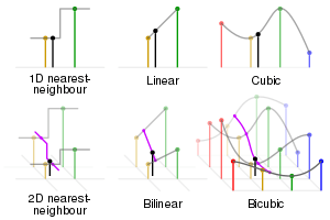
Comparison of Bicubic interpolation with some 1- and 2-dimensional interpolations. Black and red/yellow/green/blue dots correspond to the interpolated point and neighbouring samples, respectively. Their heights above the ground correspond to their values.

In mathematics, bicubic interpolation is an extension of cubic interpolation for interpolating data points on a two dimensional regular grid. The interpolated surface is smoother than corresponding surfaces obtained by bilinear interpolation or nearest-neighbor interpolation. Bicubic interpolation can be accomplished using either Lagrange polynomials, cubic splines, or cubic convolution algorithm.

In image processing, bicubic interpolation is often chosen over bilinear interpolation or nearest neighbor in image resampling, when speed is not an issue. In contrast to bilinear interpolation, which only takes 4 pixels (2×2) into account, bicubic interpolation considers 16 pixels (4×4). Images resampled with bicubic interpolation are smoother and have fewer interpolation artifacts.

Computation

Bicubic interpolation on the square

[0,4]\times [0,4]

consisting of 16 unit squares patched together. Bicubic interpolation as per Matplotlib's implementation. Colour indicates function value. The black dots are the locations of the prescribed data being interpolated. Note how the color samples are not radially symmetric.

Bilinear interpolation on the same dataset as above. Derivatives of the surface are not continuous over the square boundaries.

Nearest-neighbor interpolation on the same dataset as above. Note that the information content in all these three examples is equivalent.

Suppose the function values $f$ and the derivatives $f_{x}$ , $f_y$ and $f_{xy}$ are known at the four corners $(0,0)$ , $(1,0)$ , $(0,1)$ , and $(1,1)$ of the unit square. The interpolated surface can then be written

p(x,y) = \sum\limits_{i=0}^3 \sum_{j=0}^3 a_{ij} x^i y^j.

The interpolation problem consists of determining the 16 coefficients $a_{ij}$ . Matching $p(x,y)$ with the function values yields four equations,

$f(0,0) = p(0,0) = a_{00}$
$f(1,0) = p(1,0) = a_{00} + a_{10} + a_{20} + a_{30}$
$f(0,1) = p(0,1) = a_{00} + a_{01} + a_{02} + a_{03}$
$f(1,1) = p(1,1) = \textstyle \sum\limits_{i=0}^3 \sum\limits_{j=0}^3 a_{ij}$

Likewise, eight equations for the derivatives in the $x$ -direction and the $y$ -direction

$f_x(0,0) = p_x(0,0) = a_{10}$
$f_x(1,0) = p_x(1,0) = a_{10} + 2a_{20} + 3a_{30}$
$f_x(0,1) = p_x(0,1) = a_{10} + a_{11} + a_{12} + a_{13}$
$f_x(1,1) = p_x(1,1) = \textstyle \sum\limits_{i=1}^3 \sum\limits_{j=0}^3 a_{ij} i$
$f_y(0,0) = p_y(0,0) = a_{01}$
$f_y(1,0) = p_y(1,0) = a_{01} + a_{11} + a_{21} + a_{31}$
$f_y(0,1) = p_y(0,1) = a_{01} + 2a_{02} + 3a_{03}$
$f_y(1,1) = p_y(1,1) = \textstyle \sum\limits_{i=0}^3 \sum\limits_{j=1}^3 a_{ij} j$

And four equations for the cross derivative $xy$ .

$f_{xy}(0,0) = p_{xy}(0,0) = a_{11}$
$f_{xy}(1,0) = p_{xy}(1,0) = a_{11} + 2a_{21} + 3a_{31}$
$f_{xy}(0,1) = p_{xy}(0,1) = a_{11} + 2a_{12} + 3a_{13}$
$f_{xy}(1,1) = p_{xy}(1,1) = \textstyle \sum\limits_{i=1}^3 \sum\limits_{j=1}^3 a_{ij} i j$

where the expressions above have used the following identities,

p_x(x,y) = \textstyle \sum\limits_{i=1}^3 \sum\limits_{j=0}^3 a_{ij} i x^{i-1} y^j

p_y(x,y) = \textstyle \sum\limits_{i=0}^3 \sum\limits_{j=1}^3 a_{ij} x^i j y^{j-1}

p_{xy}(x,y) = \textstyle \sum\limits_{i=1}^3 \sum\limits_{j=1}^3 a_{ij} i x^{i-1} j y^{j-1}

This procedure yields a surface $p(x,y)$ on the unit square $[0,1] \times [0,1]$ which is continuous and with continuous derivatives. Bicubic interpolation on an arbitrarily sized regular grid can then be accomplished by patching together such bicubic surfaces, ensuring that the derivatives match on the boundaries.

Grouping the unknown parameters $a_{ij}$ in a vector,

\alpha=\left[\begin{smallmatrix}a_{00}&a_{10}&a_{20}&a_{30}&a_{01}&a_{11}&a_{21}&a_{31}&a_{02}&a_{12}&a_{22}&a_{32}&a_{03}&a_{13}&a_{23}&a_{33}\end{smallmatrix}\right]^T

and letting

x=\left[\begin{smallmatrix}f(0,0)&f(1,0)&f(0,1)&f(1,1)&f_x(0,0)&f_x(1,0)&f_x(0,1)&f_x(1,1)&f_y(0,0)&f_y(1,0)&f_y(0,1)&f_y(1,1)&f_{xy}(0,0)&f_{xy}(1,0)&f_{xy}(0,1)&f_{xy}(1,1)\end{smallmatrix}\right]^T

the above system of equations can be reformulated into a matrix for the linear equation $A\alpha=x$ .

Inverting the matrix gives the more useful linear equation $A^{{-1}}x=\alpha$ which allows $\alpha$ to be calculated quickly and easily, where:

A^{-1}=\left[\begin{smallmatrix} 1 & 0 & 0 & 0 & 0 & 0 & 0 & 0 & 0 & 0 & 0 & 0 & 0 & 0 & 0 & 0 \\ 0 & 0 & 0 & 0 & 1 & 0 & 0 & 0 & 0 & 0 & 0 & 0 & 0 & 0 & 0 & 0 \\ -3 & 3 & 0 & 0 & -2 & -1 & 0 & 0 & 0 & 0 & 0 & 0 & 0 & 0 & 0 & 0 \\ 2 & -2 & 0 & 0 & 1 & 1 & 0 & 0 & 0 & 0 & 0 & 0 & 0 & 0 & 0 & 0 \\ 0 & 0 & 0 & 0 & 0 & 0 & 0 & 0 & 1 & 0 & 0 & 0 & 0 & 0 & 0 & 0 \\ 0 & 0 & 0 & 0 & 0 & 0 & 0 & 0 & 0 & 0 & 0 & 0 & 1 & 0 & 0 & 0 \\ 0 & 0 & 0 & 0 & 0 & 0 & 0 & 0 & -3 & 3 & 0 & 0 & -2 & -1 & 0 & 0 \\ 0 & 0 & 0 & 0 & 0 & 0 & 0 & 0 & 2 & -2 & 0 & 0 & 1 & 1 & 0 & 0 \\ -3 & 0 & 3 & 0 & 0 & 0 & 0 & 0 & -2 & 0 & -1 & 0 & 0 & 0 & 0 & 0 \\ 0 & 0 & 0 & 0 & -3 & 0 & 3 & 0 & 0 & 0 & 0 & 0 & -2 & 0 & -1 & 0 \\ 9 & -9 & -9 & 9 & 6 & 3 & -6 & -3 & 6 & -6 & 3 & -3 & 4 & 2 & 2 & 1 \\ -6 & 6 & 6 & -6 & -3 & -3 & 3 & 3 & -4 & 4 & -2 & 2 & -2 & -2 & -1 & -1 \\ 2 & 0 & -2 & 0 & 0 & 0 & 0 & 0 & 1 & 0 & 1 & 0 & 0 & 0 & 0 & 0 \\ 0 & 0 & 0 & 0 & 2 & 0 & -2 & 0 & 0 & 0 & 0 & 0 & 1 & 0 & 1 & 0 \\ -6 & 6 & 6 & -6 & -4 & -2 & 4 & 2 & -3 & 3 & -3 & 3 & -2 & -1 & -2 & -1 \\ 4 & -4 & -4 & 4 & 2 & 2 & -2 & -2 & 2 & -2 & 2 & -2 & 1 & 1 & 1 & 1 \end{smallmatrix}\right]

There can be another concise matrix form for 16 coefficients

{\begin{bmatrix}f(0,0)&f(0,1)&f_{y}(0,0)&f_{y}(0,1)\\f(1,0)&f(1,1)&f_{y}(1,0)&f_{y}(1,1)\\f_{x}(0,0)&f_{x}(0,1)&f_{{xy}}(0,0)&f_{{xy}}(0,1)\\f_{x}(1,0)&f_{x}(1,1)&f_{{xy}}(1,0)&f_{{xy}}(1,1)\end{bmatrix}}={\begin{bmatrix}1&0&0&0\\1&1&1&1\\0&1&0&0\\0&1&2&3\end{bmatrix}}{\begin{bmatrix}a_{{00}}&a_{{01}}&a_{{02}}&a_{{03}}\\a_{{10}}&a_{{11}}&a_{{12}}&a_{{13}}\\a_{{20}}&a_{{21}}&a_{{22}}&a_{{23}}\\a_{{30}}&a_{{31}}&a_{{32}}&a_{{33}}\end{bmatrix}}{\begin{bmatrix}1&1&0&0\\0&1&1&1\\0&1&0&2\\0&1&0&3\end{bmatrix}}

, or

${\begin{bmatrix}a_{{00}}&a_{{01}}&a_{{02}}&a_{{03}}\\a_{{10}}&a_{{11}}&a_{{12}}&a_{{13}}\\a_{{20}}&a_{{21}}&a_{{22}}&a_{{23}}\\a_{{30}}&a_{{31}}&a_{{32}}&a_{{33}}\end{bmatrix}}={\begin{bmatrix}1&0&0&0\\0&0&1&0\\-3&3&-2&-1\\2&-2&1&1\end{bmatrix}}{\begin{bmatrix}f(0,0)&f(0,1)&f_{y}(0,0)&f_{y}(0,1)\\f(1,0)&f(1,1)&f_{y}(1,0)&f_{y}(1,1)\\f_{x}(0,0)&f_{x}(0,1)&f_{{xy}}(0,0)&f_{{xy}}(0,1)\\f_{x}(1,0)&f_{x}(1,1)&f_{{xy}}(1,0)&f_{{xy}}(1,1)\end{bmatrix}}{\begin{bmatrix}1&0&-3&2\\0&0&3&-2\\0&1&-2&1\\0&0&-1&1\end{bmatrix}}$ where $p(x,y)={\begin{bmatrix}1&x&x^{2}&x^{3}\end{bmatrix}}{\begin{bmatrix}a_{00}&a_{01}&a_{02}&a_{03}\\a_{10}&a_{11}&a_{12}&a_{13}\\a_{20}&a_{21}&a_{22}&a_{23}\\a_{30}&a_{31}&a_{32}&a_{33}\end{bmatrix}}{\begin{bmatrix}1\\y\\y^{2}\\y^{3}\end{bmatrix}}$ .

Finding derivatives from function values

If the derivatives are unknown, they are typically approximated from the function values at points neighbouring the corners of the unit square, e.g. using finite differences.

To find either of the single derivatives, $f_{x}$ or $f_y$ , using that method, find the slope between the two surrounding points in the appropriate axis. For example, to calculate $f_{x}$ for one of the points, find $f(x,y)$ for the points to the left and right of the target point and calculate their slope, and similarly for $f_y$ .

To find the cross derivative, $f_{xy}$ , take the derivative in both axes, one at a time. For example, one can first use the $f_{x}$ procedure to find the $x$ derivatives of the points above and below the target point, then use the $f_y$ procedure on those values (rather than, as usual, the values of $f$ for those points) to obtain the value of $f_{{xy}}(x,y)$ for the target point. (Or one can do it in the opposite direction, first calculating $f_y$ and then $f_{x}$ off of those. The two give equivalent results.)

At the edges of the dataset, when one is missing some of the surrounding points, the missing points can be approximated by a number of methods. A simple and common method is to assume that the slope from the existing point to the target point continues without further change, and using this to calculate a hypothetical value for the missing point.

Bicubic convolution algorithm

Bicubic spline interpolation requires the solution of the linear system described above for each grid cell. An interpolator with similar properties can be obtained by applying a convolution with the following kernel in both dimensions:

W(x) = \begin{cases} (a+2)|x|^3-(a+3)|x|^2+1 & \text{for } |x| \leq 1 \\ a|x|^3-5a|x|^2+8a|x|-4a & \text{for } 1 < |x| < 2 \\ 0 & \text{otherwise} \end{cases}

where $a$ is usually set to -0.5 or -0.75. Note that $W(0)=1$ and $W(n)=0$ for all nonzero integers $n$ .

This approach was proposed by Keys who showed that $a=-0.5$ (which corresponds to cubic Hermite spline) produces third-order convergence with respect to the sampling interval of the original function.^[1]

If we use the matrix notation for the common case $a=-0.5$ , we can express the equation in a more friendly manner:

p(t)={\tfrac {1}{2}}{\begin{bmatrix}1&t&t^{2}&t^{3}\\\end{bmatrix}}{\begin{bmatrix}0&2&0&0\\-1&0&1&0\\2&-5&4&-1\\-1&3&-3&1\\\end{bmatrix}}{\begin{bmatrix}f_{-1}\\f_{0}\\f_{1}\\f_{2}\\\end{bmatrix}}

for $t$ between 0 and 1 for one dimension. Note that for 1-dimensional cubic convolution interpolation 4 sample points are required. For each inquiry two samples are located on its left and two samples on the right. These points are indexed from -1 to 2 in this text. The distance from the point indexed with 0 to the inquiry point is denoted by $t$ here.

For two dimensions first applied once in $x$ and again in $y$ :

\textstyle b_{-1}=p(t_{x},f_{(-1,-1)},f_{(0,-1)},f_{(1,-1)},f_{(2,-1)})

\textstyle b_{0}=p(t_{x},f_{(-1,0)},f_{(0,0)},f_{(1,0)},f_{(2,0)})

\textstyle b_{1}=p(t_{x},f_{(-1,1)},f_{(0,1)},f_{(1,1)},f_{(2,1)})

\textstyle b_{2}=p(t_{x},f_{(-1,2)},f_{(0,2)},f_{(1,2)},f_{(2,2)})

\textstyle p(x,y) = p(t_y, b_{-1}, b_{0}, b_{1}, b_{2})

Use in computer graphics

The lower half of this figure is a magnification of the upper half, showing how the apparent sharpness of the left-hand line is created. Bicubic interpolation causes overshoot, which increases acutance.

The bicubic algorithm is frequently used for scaling images and video for display (see bitmap resampling). It preserves fine detail better than the common bilinear algorithm.

However, due to the negative lobes on the kernel, it causes overshoot (haloing). This can cause clipping, and is an artifact (see also ringing artifacts), but it increases acutance (apparent sharpness), and can be desirable.

References

↑ R. Keys, (1981). "Cubic convolution interpolation for digital image processing". IEEE Transactions on Acoustics, Speech, and Signal Processing. 29 (6): 1153–1160. doi:10.1109/TASSP.1981.1163711.

External links

This article is issued from Wikipedia - version of the 11/28/2016. The text is available under the Creative Commons Attribution/Share Alike but additional terms may apply for the media files.