Stiff equation

In mathematics, a stiff equation is a differential equation for which certain numerical methods for solving the equation are numerically unstable, unless the step size is taken to be extremely small. It has proven difficult to formulate a precise definition of stiffness, but the main idea is that the equation includes some terms that can lead to rapid variation in the solution.

When integrating a differential equation numerically, one would expect the requisite step size to be relatively small in a region where the solution curve displays much variation and to be relatively large where the solution curve straightens out to approach a line with slope nearly zero. For some problems this is not the case. Sometimes the step size is forced down to an unacceptably small level in a region where the solution curve is very smooth. The phenomenon being exhibited here is known as stiffness. In some cases we may have two different problems with the same solution, yet problem one is not stiff and problem two is stiff. Clearly the phenomenon cannot be a property of the exact solution, since this is the same for both problems, and must be a property of the differential system itself. It is thus appropriate to speak of stiff systems.

Motivating example

Explicit numerical methods exhibiting instability when integrating a stiff ordinary differential equation

Consider the initial value problem

$\,y'(t)=-15y(t),\quad t\geq 0,y(0)=1.$

(1)

The exact solution (shown in cyan) is

$y(t)=e^{-15t}\,$ with $y(t)\to 0$ as $t\to \infty .$

(2)

We seek a numerical solution that exhibits the same behavior.

The figure (right) illustrates the numerical issues for various numerical integrators applied on the equation.

Euler's method with a step size of h = 1/4 oscillates wildly and quickly exits the range of the graph (shown in red).
Euler's method with half the step size, h = 1/8, produces a solution within the graph boundaries, but oscillates about zero (shown in green).
The trapezoidal method (that is, the two-stage Adams–Moulton method) is given by

$y_{n+1}=y_{n}+{\frac {1}{2}}h\left(f(t_{n},y_{n})+f(t_{n+1},y_{n+1})\right),$

(3)

where $\textstyle y'=f(t,y)$ . Applying this method instead of Euler's method gives a much better result (blue). The numerical results decrease monotonically to zero, just as the exact solution does.

One of the most prominent examples of the stiff ODEs is a system that describes the chemical reaction of Robertson:

${\dot {x}}=-0.04x+10^{4}y\cdot z$
${\dot {y}}=0.04x-10^{4}y\cdot z-3\cdot 10^{7}y^{2}$
${\dot {z}}=3\cdot 10^{7}y^{2}$

(4)

If one treats this system on a short interval, for example, $t\in [0,40]$ there is no problem in numerical integration. However, if the interval is very large (10¹¹ say), then many standard codes fail to integrate it correctly.

Additional examples are the sets of ODEs resulting from the temporal integration of large chemical reaction mechanisms. Here, the stiffness arises from the coexistence of very slow and very fast reactions. To solve them, the software packages KPP and Autochem can be used.

Stiffness ratio

Consider the linear constant coefficient inhomogeneous system

${\mathbf {y}}'={\mathbf {A}}{\mathbf {y}}+{\mathbf {f}}(x),$

(5)

where ${\mathbf {y}},{\mathbf {f}}\in \mathbb {R} ^{n}$ and ${\mathbf {A}}$ is a constant $n\times n$ matrix with eigenvalues $\lambda _{t}\in \mathbb {C} ,t=1,2,\ldots ,n$ (assumed distinct) and corresponding eigenvectors ${\mathbf {c}}_{t}\in \mathbb {C} ^{n},t=1,2,\ldots ,n$ . The general solution of (5) takes the form

${\mathbf {y}}(x)=\sum _{t=1}^{n}\kappa _{t}\exp(\lambda _{t}x){\mathbf {c}}_{t}+{\mathbf {g}}(x),$

(6)

where the κ_t are arbitrary constants and ${\mathbf {g}}(x)$ is a particular integral. Now let us suppose that

$Re(\lambda _{t})<0,\qquad t=1,2,\ldots ,n,$

(7)

which implies that each of the terms $\exp(\lambda _{t}x){\mathbf {c}}_{t}\rightarrow 0$ as $x\rightarrow \infty$ , so that the solution ${\mathbf {y}}(x)$ approaches ${\mathbf {g}}(x)$ asymptotically as $x\rightarrow \infty$ ; the term $\exp(\lambda _{t}x){\mathbf {c}}_{t}$ will decay monotonically if λ_t is real and sinusoidally if λ_t is complex. Interpreting x to be time (as it often is in physical problems) it is appropriate to call $\Sigma _{t=1}^{n}\kappa _{t}\exp(\lambda _{t}x){\mathbf {c}}_{t}$ the transient solution and ${\mathbf {g}}(x)$ the steady-state solution. If $|Re(\lambda _{t})|$ is large, then the corresponding term $\kappa _{t}\exp(\lambda _{t}x){\mathbf {c}}_{t}$ will decay quickly as x increases and is thus called a fast transient; if $|Re(\lambda _{t})|$ is small, the corresponding term $\kappa _{t}\exp(\lambda _{t}x){\mathbf {c}}_{t}$ decays slowly and is called a slow transient. Let ${\overline {\lambda }},{\underline {\lambda }}\in \{\lambda _{t},t=1,2,\ldots ,n\}$ be defined by

$|Re({\overline {\lambda }})|\geq |Re(\lambda _{t})|\geq |Re({\underline {\lambda }})|,\qquad t=1,2,\ldots ,n$

(8)

so that $\kappa _{t}\exp({\overline {\lambda }}x){\mathbf {c}}_{t}$ is the fastest transient and $\kappa _{t}\exp({\underline {\lambda }}x){\mathbf {c}}_{t}$ the slowest. We now define the stiffness ratio as

${\frac {|Re({\overline {\lambda }})|}{|Re({\underline {\lambda }})|}}.$ ^[1]

(9)

Characterization of stiffness

In this section we consider various aspects of the phenomenon of stiffness. 'Phenomenon' is probably a more appropriate word than 'property', since the latter rather implies that stiffness can be defined in precise mathematical terms; it turns out not to be possible to do this in a satisfactory manner, even for the restricted class of linear constant coefficient systems. We shall also see several qualitative statements that can be (and mostly have been) made in an attempt to encapsulate the notion of stiffness, and state what is probably the most satisfactory of these as a 'definition' of stiffness.

J. D. Lambert defines stiffness as follows:

If a numerical method with a finite region of absolute stability, applied to a system with any initial conditions, is forced to use in a certain interval of integration a steplength which is excessively small in relation to the smoothness of the exact solution in that interval, then the system is said to be stiff in that interval.

There are other characteristics which are exhibited by many examples of stiff problems, but for each there are counterexamples, so these characteristics do not make good definitions of stiffness. Nonetheless, definitions based upon these characteristics are in common use by some authors and are good clues as to the presence of stiffness. Lambert refers to these as 'statements' rather than definitions, for the aforementioned reasons. A few of these are:

A linear constant coefficient system is stiff if all of its eigenvalues have negative real part and the stiffness ratio is large.
Stiffness occurs when stability requirements, rather than those of accuracy, constrain the steplength.
Stiffness occurs when some components of the solution decay much more rapidly than others.^[2]

Etymology

The origin of the term 'stiffness' seems to be somewhat of a mystery. According to Joseph Oakland Hirschfelder, the term 'stiff' is used because such systems correspond to tight coupling between the driver and driven in servomechanisms.^[3] According to Richard. L. Burden and J. Douglas Faires,

Significant difficulties can occur when standard numerical techniques are applied to approximate the solution of a differential equation when the exact solution contains terms of the form e^λt, where λ is a complex number with negative real part.
...
Problems involving rapidly decaying transient solutions occur naturally in a wide variety of applications, including the study of spring and damping systems, the analysis of control systems, and problems in chemical kinetics. These are all examples of a class of problems called stiff (mathematical stiffness) systems of differential equations, due to their application in analyzing the motion of spring and mass systems having large spring constants (physical stiffness).^[4]

For example, the initial value problem

$m{\ddot {x}}+c{\dot {x}}+kx=0,\qquad x(0)=x_{0},\qquad {\dot {x}}(0)=0,$

(10)

with m = 1, c = 1001, k = 1000, can be written in the form (5) with n = 2 and

${\mathbf {A}}=\left({\begin{array}{rr}0&1\\-1000&-1001\end{array}}\right),$

(11)

${\mathbf {f}}(t)=\left({\begin{array}{c}0\\0\end{array}}\right),$

(12)

${\mathbf {x}}(0)=\left({\begin{array}{c}x_{0}\\0\end{array}}\right),$

(13)

and has eigenvalues ${\overline {\lambda }}=-1000,{\underline {\lambda }}=-1$ . Both eigenvalues have negative real part and the stiffness ratio is

${\frac {|-1000|}{|-1|}}=1000,$

(14)

which is fairly large. System (10) then certainly satisfies statements 1 and 3. Here the spring constant k is large and the damping constant c is even larger.^[5] (Note that 'large' is a vague, subjective term, but the larger the above quantities are, the more pronounced will be the effect of stiffness.) The exact solution to (10) is

$x(t)=x_{0}\left(-{\frac {1}{999}}e^{-1000t}+{\frac {1000}{999}}e^{-t}\right)\approx x_{0}e^{-t}.$

(15)

Note that (15) behaves quite nearly as a simple exponential x₀e^−t, but the presence of the e^−1000t term, even with a small coefficient is enough to make the numerical computation very sensitive to step size. Stable integration of (10) requires a very small step size until well into the smooth part of the solution curve, resulting in an error much smaller than required for accuracy. Thus the system also satisfies statement 2 and Lambert's definition.

A-stability

The behaviour of numerical methods on stiff problems can be analyzed by applying these methods to the test equation $y' = ky$ subject to the initial condition $y (0) = 1$ with $k\in \mathbb {C}$ . The solution of this equation is $y (t) = e kt$ . This solution approaches zero as $t\to \infty$ when $\mathrm {Re} \,(k)<0.$ If the numerical method also exhibits this behaviour (for a fixed step size), then the method is said to be A-stable.^[6] (Note that a numerical method that is L-stable (see below) has the stronger property that the solution approaches zero in a single step as the step size goes to infinity.) A-stable methods do not exhibit the instability problems as described in the motivating example.

Runge–Kutta methods

Runge–Kutta methods applied to the test equation $y'=k\cdot y$ take the form $y_{n+1}=\phi (hk)\cdot y_{n}$ , and, by induction, $y_{n}=\left(\phi (hk)\right)^{n}\cdot y_{0}$ . The function $\phi$ is called the stability function. Thus, the condition that $y_{n}\to 0$ as $n\to \infty$ is equivalent to $|\phi (hk)|<1$ . This motivates the definition of the region of absolute stability (sometimes referred to simply as stability region), which is the set $\{z\in \mathbb {C} |\,|\phi (z)|<1\}$ . The method is A-stable if the region of absolute stability contains the set $\{z\in \mathbb {C} |\mathrm {Re} (z)<0\}$ , that is, the left half plane.

Example: The Euler methods

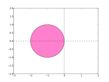
The pink disk shows the stability region for the Euler method.

Consider the Euler methods above. The explicit Euler method applied to the test equation $y'=k\cdot y$ is

y_{n+1}=y_{n}+h\cdot f(t_{n},y_{n})=y_{n}+h\cdot (ky_{n})=y_{n}+h\cdot k\cdot y_{n}=(1+h\cdot k)y_{n}.

Hence, $y_{n}=(1+hk)^{n}\cdot y_{0}$ with $\phi (z)=1+z$ . The region of absolute stability for this method is thus $\{z\in \mathbb {C} ||1+z|<1\}$ which is the disk depicted on the right. The Euler method is not A-stable.

The motivating example had $k=-15$ . The value of z when taking step size $h=1/4$ is $z=-15*1/4=-3.75$ , which is outside the stability region. Indeed, the numerical results do not converge to zero. However, with step size $h=1/8$ , we have $z=-1.875$ which is just inside the stability region and the numerical results converge to zero, albeit rather slowly.

Example: Trapezoidal method

The pink region is the stability region for the trapezoidal method.

Consider the trapezoidal method

y_{n+1}=y_{n}+{\tfrac {1}{2}}h\cdot \left(f(t_{n},y_{n})+f(t_{n+1},y_{n+1})\right),

when applied to the test equation $y'=k\cdot y$ , is

y_{n+1}=y_{n}+{\tfrac {1}{2}}h\cdot \left(ky_{n}+ky_{n+1}\right).

Solving for $y_{n+1}$ yields

y_{n+1}={\frac {1+{\frac {1}{2}}hk}{1-{\frac {1}{2}}hk}}\cdot y_{n}.

Thus, the stability function is

\phi (z)={1+{1 \over 2}z \over 1-{1 \over 2}z}

and the region of absolute stability is

\left\{z\in \mathbb {C} \left|\ \left|{1+{1 \over 2}z \over 1-{1 \over 2}z}\right|<1\right.\right\}.

This region contains the left-half plane, so the trapezoidal method is A-stable. In fact, the stability region is identical to the left-half plane, and thus the numerical solution of $y'=k\cdot y$ converges to zero if and only if the exact solution does. Nevertheless, the trapezoidal method does not have perfect behavior: it does damp all decaying components, but rapidly decaying components are damped only very mildly, because $\phi (z)\to 1$ as $z\to -\infty$ . This led to the concept of L-stability: a method is L-stable if it is A-stable and $|\phi (z)|\to 0$ as $z\to \infty$ . The trapezoidal method is A-stable but not L-stable. The implicit Euler method is an example of an L-stable method.^[7]

General theory

The stability function of a Runge–Kutta method with coefficients $A$ and $b$ is given by

\phi (z)={\frac {\det(I-zA+zeb^{T})}{\det(I-zA)}},

where $e$ denotes the vector with ones. This is a rational function (one polynomial divided by another).

Explicit Runge–Kutta methods have a strictly lower triangular coefficient matrix $A$ and thus, their stability function is a polynomial. It follows that explicit Runge–Kutta methods cannot be A-stable.

The stability function of implicit Runge–Kutta methods is often analyzed using order stars. The order star for a method with stability function $\phi$ is defined to be the set $\{z\in \mathbb {C} ||\phi (z)|>|\mathrm {e} ^{z}|\}$ . A method is A-stable if and only if its stability function has no poles in the left-hand plane and its order star contains no purely imaginary numbers.^[8]

Multistep methods

Linear multistep methods have the form

y_{n+1}=\sum _{i=0}^{s}a_{i}y_{n-i}+h\sum _{j=-1}^{s}b_{j}f(t_{n-j},y_{n-j}).

Applied to the test equation, they become

y_{n+1}=\sum _{i=0}^{s}a_{i}y_{n-i}+hk\sum _{j=-1}^{s}b_{j}y_{n-j},

which can be simplified to

(1-b_{-1}z)y_{n+1}-\sum _{j=0}^{s}(a_{j}+b_{j}z)y_{n-j}=0

where z = hk. This is a linear recurrence relation. The method is A-stable if all solutions {y_n} of the recurrence relation converge to zero when Re z < 0. The characteristic polynomial is

\Phi (z,w)=w^{s+1}-\sum _{i=0}^{s}a_{i}w^{s-i}-z\sum _{j=-1}^{s}b_{j}w^{s-j}.

All solutions converge to zero for a given value of z if all solutions w of Φ(z,w) = 0 lie in the unit circle.

The region of absolute stability for a multistep method of the above form is then the set of all $z\in \mathbb {C}$ for which all w such that Φ(z,w) = 0 satisfy |w| < 1. Again, if this set contains the left-half plane, the multi-step method is said to be A-stable.

Example: The second-order Adams–Bashforth method

The pink region is the stability region for the second-order Adams–Bashforth method.

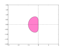
Let us determine the region of absolute stability for the two-step Adams–Bashforth method

y_{n+1}=y_{n}+h\left({\tfrac {3}{2}}f(t_{n},y_{n})-{\tfrac {1}{2}}f(t_{n-1},y_{n-1})\right).

The characteristic polynomial is

\Phi (w,z)=w^{2}-(1+{\tfrac {3}{2}}z)w+{\tfrac {1}{2}}z=0

which has roots

w={\tfrac {1}{2}}{\Big (}1+{\tfrac {3}{2}}z\pm {\sqrt {1+z+{\tfrac {9}{4}}z^{2}}}{\Big )},

thus the region of absolute stability is

\left\{z\in \mathbb {C} \left|\ \left|{\tfrac {1}{2}}{\Big (}1+{\tfrac {3}{2}}z\pm {\sqrt {1+z+{\tfrac {9}{4}}z^{2}}}{\Big )}\right|<1\right.\right\}.

This region is shown on the right. It does not include all the left half-plane (in fact it only includes the real axis between z = −1 and z = 0) so the Adams–Bashforth method is not A-stable.

General theory

Explicit multistep methods can never be A-stable, just like explicit Runge–Kutta methods. Implicit multistep methods can only be A-stable if their order is at most 2. The latter result is known as the second Dahlquist barrier; it restricts the usefulness of linear multistep methods for stiff equations. An example of a second-order A-stable method is the trapezoidal rule mentioned above, which can also be considered as a linear multistep method.^[9]

Notes

↑ Lambert (1992, pp. 216–217)
↑ Lambert (1992, pp. 217–220)
↑ Hirshfelder (1963)
↑ Burden & Faires (1993, p. 314)
↑ Kreyszig (1972, pp. 62–68)
↑ This definition is due to Dahlquist (1963).
↑ The definition of L-stability is due to Ehle (1969).
↑ The definition is due to Wanner, Hairer & Nørsett (1978); see also Iserles & Nørsett (1991).
↑ See Dahlquist (1963).

References

Burden, Richard L.; Faires, J. Douglas (1993), Numerical Analysis (5th ed.), Boston: Prindle, Weber and Schmidt, ISBN 0-534-93219-3 .
Dahlquist, Germund (1963), "A special stability problem for linear multistep methods", BIT, 3 (1): 27–43, doi:10.1007/BF01963532 .
Eberly, David (2008), Stability analysis for systems of differential equations .
Ehle, B. L. (1969), On Padé approximations to the exponential function and A-stable methods for the numerical solution of initial value problems, Report 2010, University of Waterloo .
Gear, C. W. (1971), Numerical Initial-Value Problems in Ordinary Differential Equations, Englewood Cliffs: Prentice Hall .
Gear, C. W. (1981), "Numerical solution of ordinary differential equations: Is there anything left to do?", SIAM Review, 23 (1): 10–24 .
Hairer, Ernst; Wanner, Gerhard (1996), Solving ordinary differential equations II: Stiff and differential-algebraic problems (second ed.), Berlin: Springer-Verlag, ISBN 978-3-540-60452-5 .
Hirshfelder, J. O. (1963), "Applied Mathematics as used in Theoretical Chemistry", American Mathematical Society Symposium: 367–376 .
Iserles, Arieh; Nørsett, Syvert (1991), Order Stars, Chapman & Hall, ISBN 978-0-412-35260-7 .
Kreyszig, Erwin (1972), Advanced Engineering Mathematics (3rd ed.), New York: Wiley, ISBN 0-471-50728-8 .
Lambert, J. D. (1977), D. Jacobs, ed., "The initial value problem for ordinary differential equations", The State of the Art in Numerical Analysis, New York: Academic Press: 451–501 .
Lambert, J. D. (1992), Numerical Methods for Ordinary Differential Systems, New York: Wiley, ISBN 978-0-471-92990-1 .
Mathews, John; Fink, Kurtis (1992), Numerical methods using MATLAB .
Press, WH; Teukolsky, SA; Vetterling, WT; Flannery, BP (2007). "Section 17.5. Stiff Sets of Equations". Numerical Recipes: The Art of Scientific Computing (3rd ed.). New York: Cambridge University Press. ISBN 978-0-521-88068-8.
Shampine, L. F.; Gear, C. W. (1979), "A user's view of solving stiff ordinary differential equations", SIAM Review, 21 (1): 1–17 .
Wanner, Gerhard; Hairer, Ernst; Nørsett, Syvert (1978), "Order stars and stability theory", BIT, 18 (4): 475–489, doi:10.1007/BF01932026 .
Stability of Runge-Kutta Methods

External links

An Introduction to Physically Based Modeling: Energy Functions and Stiffness
Stiff systems Lawrence F. Shampine and Skip Thompson Scholarpedia, 2(3):2855. doi:10.4249/scholarpedia.2855

This article is issued from Wikipedia - version of the 6/10/2016. The text is available under the Creative Commons Attribution/Share Alike but additional terms may apply for the media files.

Stiff equation

Motivating example

Stiffness ratio

Characterization of stiffness

Etymology

A-stability

Runge–Kutta methods

Example: The Euler methods

Example: Trapezoidal method

General theory

Multistep methods

Example: The second-order Adams–Bashforth method

General theory

See also

Notes

References

External links