Quadratic formula

The quadratic formula

In elementary algebra, the quadratic formula is the solution of the quadratic equation. There are other ways to solve the quadratic equation instead of using the quadratic formula, such as factoring, completing the square, or graphing. Using the quadratic formula is often the most convenient way.

The general quadratic equation is

ax^{2}+bx+c=0.

Here $x$ represents an unknown, while $a$ , $b$ , and $c$ are constants with $a$ not equal to 0. One can verify that the quadratic formula satisfies the quadratic equation, by inserting the former into the latter. With the above parameterization, the quadratic formula is:

x={\frac {-b\pm {\sqrt {b^{2}-4ac}}}{2a}}.

Each of the solutions given by the quadratic formula is called a root of the quadratic equation. Geometrically, these roots represent the $x$ values at which any parabola, explicitly given as $y = ax 2 + bx + c$ , crosses the $x$ -axis. As well as being a formula that will yield the zeros of any parabola, the quadratic equation will give the axis of symmetry of the parabola, and it can be used to immediately determine how many zeros it has.

Derivation of the formula

The quadratic formula can be derived with a simple application of technique of completing the square.^[1]^[2] For this reason, the derivation is sometimes left as an exercise for students, who can thus experience rediscovery of this important formula.^[3]^[4] The explicit derivation is as follows.

Divide the quadratic equation by $a$ , which is allowed because $a$ is non-zero:

x^{2}+{\frac {b}{a}}x+{\frac {c}{a}}=0.

Subtract $c / a$ from both sides of the equation, yielding:

x^{2}+{\frac {b}{a}}x=-{\frac {c}{a}}.

The quadratic equation is now in a form to which the method of completing the square can be applied. Thus, add a constant to both sides of the equation such that the left hand side becomes a complete square:

x^{2}+{\frac {b}{a}}x+\left({\frac {b}{2a}}\right)^{2}=-{\frac {c}{a}}+\left({\frac {b}{2a}}\right)^{2},

which produces:

\left(x+{\frac {b}{2a}}\right)^{2}=-{\frac {c}{a}}+{\frac {b^{2}}{4a^{2}}}.

Accordingly, after rearranging the terms on the right hand side to have a common denominator, we obtain this:

\left(x+{\frac {b}{2a}}\right)^{2}={\frac {b^{2}-4ac}{4a^{2}}}.

The square has thus been completed. Taking the square root of both sides yields the following equation:

x+{\frac {b}{2a}}=\pm {\frac {\sqrt {b^{2}-4ac\ }}{2a}}.

Isolating $x$ gives the quadratic formula:

x={\frac {-b\pm {\sqrt {b^{2}-4ac\ }}}{2a}}.

The plus-minus symbol "±" indicates that both

x={\frac {-b+{\sqrt {b^{2}-4ac}}}{2a}}\quad {\text{and}}\quad x={\frac {-b-{\sqrt {b^{2}-4ac}}}{2a}}

are solutions of the quadratic equation.^[5] There are many alternatives of this derivation with minor differences, mostly concerning the manipulation of $a$ .

Some sources, particularly older ones, use alternative parameterizations of the quadratic equation such as $ax 2 - 2 bx + c = 0$ ^[6] or $ax 2 + 2 bx + c = 0$ ,^[7] where $b$ has a magnitude one half of the more common one. These result in slightly different forms for the solution, but are otherwise equivalent.

A lesser known quadratic formula, as used in Muller's method, and which can be found from Vieta's formulas, provides the same roots via the equation:

x={\frac {-2c}{b\pm {\sqrt {b^{2}-4ac}}}}.

Geometrical significance

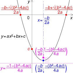
Graph of y = ax² + bx + c, where a and the discriminant (b² - 4ac) are positive, with

Roots and y-intercept in red
Vertex and axis of symmetry in blue
Focus and directrix in pink

Visualisation of the complex roots of y = ax² + bx + c : the parabola is rotated 180° about its vertex (yellow). Its x-intercepts are rotated 90° around their mid-point, and the Cartesian plane is interpreted as the complex plane (green).^[8]

Without going into parabolas as geometrical objects on a cone (see Conic section), a parabola is any curve described by a second-degree polynomial, i.e. any equation of the form:

p(x)=a_{2}x^{2}+a_{1}x+a_{0}

where $p$ represents the polynomial of degree 2 and $a 0, a 1,$ and $a 2$ are constant coefficients whose subscripts correspond to their respective term's degree. The first and foremost geometrical application of the quadratic formula is that it will define the points along the $x$ -axis where the parabola will cross it. Additionally, if the quadratic formula were broken into two terms,

x={\frac {-b\pm {\sqrt {b^{2}-4ac\ }}}{2a}}=-{\frac {b}{2a}}\pm {\frac {\sqrt {b^{2}-4ac\ }}{2a}}

the definition of the axis of symmetry appears as the $- b / 2 a$ term. The other term, $\sqrt b 2 - 4 ac / 2 a$ , must then be the distance the zeros are away from the axis of symmetry, where the plus sign represents the distance away to the right, and the minus sign represents the distance away to the left.

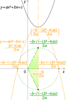
If this distance term were to decrease to zero, the axis of symmetry would be the $x$ value of the zero, indicating there is only one possible solution to the quadratic equation. Algebraically, this means that $\sqrt b 2 - 4 ac = 0$ , or simply $b 2 - 4 ac = 0$ (where the left-hand side is referred to as the discriminant), for its term to be reduced to zero. This is simply one of three cases, where the discriminant can indicate how many zeros the parabola will have. If the discriminant were positive, the distance would be non-zero, and there will be two solutions, as expected. However, there is the case where the discriminant is less than zero, and this indicates the distance will be imaginary — or some multiple of the unit $i$ , such that $i = \sqrt -1$ — and the parabola's zeros will be a complex number. The complex roots will be complex conjugates, and by definition cannot be entirely real, where the real part of the complex root will be the axis of symmetry, therefore geometrical interpretation is that there are no real values of $x$ such that the parabola will be observed to cross the $x$ -axis.

Historical development

The earliest methods for solving quadratic equations were geometric. Babylonian cuneiform tablets contain problems reducible to solving quadratic equations.^[9] The Egyptian Berlin Papyrus, dating back to the Middle Kingdom (2050 BC to 1650 BC), contains the solution to a two-term quadratic equation.^[10]

Euclid in Raphael's School of Athens

The Greek mathematician Euclid (circa 300 BC) used geometric methods to solve quadratic equations in Book 2 of his Elements, an influential mathematical treatise.^[11] Rules for quadratic equations appear in the Chinese The Nine Chapters on the Mathematical Art circa 200 BC.^[12]^[13] In his work Arithmetica, the Greek mathematician Diophantus (circa 250 BC) solved quadratic equations with a method more recognizably algebraic than the geometric algebra of Euclid.^[11] His solution gives only one root, even when both roots are positive.^[14]

The Indian mathematician Brahmagupta (597–668 AD) explicitly described the quadratic formula in his treatise Brāhmasphuṭasiddhānta published in 628 AD,^[15] but written in words instead of symbols.^[16] His solution of the quadratic equation $ax 2 + bx = c$ was as follows: "To the absolute number multiplied by four times the [coefficient of the] square, add the square of the [coefficient of the] middle term; the square root of the same, less the [coefficient of the] middle term, being divided by twice the [coefficient of the] square is the value."^[17] This is equivalent to:

x={\frac {{\sqrt {4ac+b^{2}}}-b}{2a}}.

The 9th-century Persian mathematician al-Khwārizmī, influenced by earlier Greek and Indian mathematicians, solved quadratic equations algebraically.^[18] The quadratic formula covering all cases was first obtained by Simon Stevin in 1594.^[19] In 1637 René Descartes published La Géométrie containing the quadratic formula in the form we know today. The first appearance of the general solution in the modern mathematical literature appeared in an 1896 paper by Henry Heaton.^[20]

Other derivations

Many alternative derivations of the quadratic formula are in the literature. These derivations may be simpler than the standard completing the square method, may represent interesting applications of other alegraic techniques, or may offer insight into other areas of mathematics.

Alternate method of completing the square

The great majority of algebra texts published over the last several decades teach completing the square using the sequence presented earlier: (1) divide each side by $a$ to make the equation monic, (2) rearrange, (3) then add $(b / 2 a) 2$ to both sides to complete the square.

As pointed out by Larry Hoehn in 1975, completing the square can be accomplished by a different sequence that leads to a simpler sequence of intermediate terms: (1) multiply each side by $4 a$ , (2) rearrange, (3) then add $b 2$ .^[21]

In other words, the quadratic formula can be derived as follows:

{\begin{aligned}ax^{2}+bx+c&=0\\4a^{2}x^{2}+4abx+4ac&=0\\4a^{2}x^{2}+4abx&=-4ac\\4a^{2}x^{2}+4abx+b^{2}&=b^{2}-4ac\\(2ax+b)^{2}&=b^{2}-4ac\\2ax+b&=\pm {\sqrt {b^{2}-4ac}}\\2ax&=-b\pm {\sqrt {b^{2}-4ac}}\\x&={\frac {-b\pm {\sqrt {b^{2}-4ac}}}{2a}}.\\\end{aligned}}

This actually represents an ancient derivation of the quadratic formula, and was known to the Hindus at least as far back as 1025.^[22] Compared with the derivation in standard usage, this alternate derivation is shorter, involves fewer computations with literal coefficients, avoids fractions until the last step, has simpler expressions, and uses simpler mathematics. As Hoehn states, "it is easier 'to add the square of $b$ ' than it is 'to add the square of half the coefficient of the $x$ term'".^[21]

By substitution

Another technique is solution by substitution.^[23] In this technique, we substitute $x = y + m$ into the quadratic to get:

a(y+m)^{2}+b(y+m)+c=0.

Expanding the result and then collecting the powers of $y$ produces:

ay^{2}+y(2am+b)+(am^{2}+bm+c)=0.

We have not yet imposed a second condition on $y$ and $m$ , so we now choose $m$ so that the middle term vanishes. That is, $2 am + b = 0$ or $m = - b / 2 a$ . Subtracting the constant term from both sides of the equation (to move it to the right hand side) and then dividing by $a$ gives:

y^{2}={\frac {-(am^{2}+bm+c)}{a}}.

Substituting for $m$ gives:

y^{2}={\frac {-({\frac {b^{2}}{4a}}+{\frac {-b^{2}}{2a}}+c)}{a}}={\frac {b^{2}-4ac}{4a^{2}}}.

Therefore,

y=\pm {\frac {\sqrt {b^{2}-4ac}}{2a}};

substituting $x = y + m = y - b / 2 a$ provides the quadratic formula.

By using algebraic identities

The following method was used by many historical mathematicians:^[24]

Let the roots of the standard quadratic equation be $r 1$ and $r 2$ . The derivation starts by recalling the identity:

(r_{1}-r_{2})^{2}=(r_{1}+r_{2})^{2}-4r_{1}r_{2}.

Taking the square root on both sides, we get:

r_{1}-r_{2}=\pm {\sqrt {(r_{1}+r_{2})^{2}-4r_{1}r_{2}}}.

Since the coefficient $a \neq 0$ , we can divide the standard equation by $a$ to obtain a quadratic polynomial having the same roots. Namely,

x^2 + \frac{b}{a}x + \frac{c}{a} = (x - r_1)(x-r_2) = x^2 - (r_1 + r_2)x + r_1 r_2.

From this we can see that the sum of the roots of the standard quadratic equation is given by $- b / a$ , and the product of those roots is given by $c / a$ . Hence the identity can be rewritten as:

r_{1}-r_{2}=\pm {\sqrt {\left(-{\frac {b}{a}}\right)^{2}-4{\frac {c}{a}}}}=\pm {\sqrt {{\frac {b^{2}}{a^{2}}}-{\frac {4ac}{a^{2}}}}}=\pm {\frac {\sqrt {b^{2}-4ac}}{a}}.

Now,

r_1 = \frac{(r_1 + r_2) + (r_1 - r_2)}{2} = \frac{-\frac{b}{a} \pm \frac{\sqrt{b^2 - 4ac}}{a}}{2} = \frac{-b \pm \sqrt{b^2 - 4ac}}{2a}.

Since $r 2 = - r 1 - b / a$ , if we take

r_1 = \frac{-b + \sqrt{b^2 - 4ac}}{2a}

then we obtain

r_{2}={\frac {-b-{\sqrt {b^{2}-4ac}}}{2a}};

and if we instead take

r_1 = \frac{-b - \sqrt{b^2 - 4ac}}{2a}

then we calculate that

r_2 = \frac{-b + \sqrt{b^2 - 4ac}}{2a}.

Combining these results by using the standard shorthand ±, we have that the solutions of the quadratic equation are given by:

x={\frac {-b\pm {\sqrt {b^{2}-4ac}}}{2a}}.

By Lagrange resolvents

For more details on this topic, see Lagrange resolvents.

An alternative way of deriving the quadratic formula is via the method of Lagrange resolvents,^[25] which is an early part of Galois theory.^[26] This method can be generalized to give the roots of cubic polynomials and quartic polynomials, and leads to Galois theory, which allows one to understand the solution of algebraic equations of any degree in terms of the symmetry group of their roots, the Galois group.

This approach focuses on the roots more than on rearranging the original equation. Given a monic quadratic polynomial

x^2+px+q,

assume that it factors as

x^2+px+q=(x-\alpha)(x-\beta),

Expanding yields

x^2+px+q=x^2-(\alpha+\beta)x+\alpha \beta,

where $p = -(α + β)$ and $q = αβ$ .

Since the order of multiplication does not matter, one can switch $α$ and $β$ and the values of $p$ and $q$ will not change: one can say that $p$ and $q$ are symmetric polynomials in $α$ and $β$ . In fact, they are the elementary symmetric polynomials – any symmetric polynomial in $α$ and $β$ can be expressed in terms of $α + β$ and $αβ$ The Galois theory approach to analyzing and solving polynomials is: given the coefficients of a polynomial, which are symmetric functions in the roots, can one "break the symmetry" and recover the roots? Thus solving a polynomial of degree $n$ is related to the ways of rearranging ("permuting") $n$ terms, which is called the symmetric group on $n$ letters, and denoted $S n$ . For the quadratic polynomial, the only way to rearrange two terms is to swap them ("transpose" them), and thus solving a quadratic polynomial is simple.

To find the roots $α$ and $β$ , consider their sum and difference:

\begin{align} r_1 &= \alpha + \beta\\ r_2 &= \alpha - \beta. \end{align}

These are called the Lagrange resolvents of the polynomial; notice that one of these depends on the order of the roots, which is the key point. One can recover the roots from the resolvents by inverting the above equations:

\begin{align} \alpha &= \textstyle{\frac{1}{2}}\left(r_1+r_2\right)\\ \beta &= \textstyle{\frac{1}{2}}\left(r_1-r_2\right). \end{align}

Thus, solving for the resolvents gives the original roots.

Now $r 1 = α + β$ is a symmetric function in $α$ and $β$ , so it can be expressed in terms of $p$ and $q$ , and in fact $r 1 = - p$ as noted above. But $r 2 = α - β$ is not symmetric, since switching $α$ and $β$ yields $- r 2 = β - α$ (formally, this is termed a group action of the symmetric group of the roots). Since $r 2$ is not symmetric, it cannot be expressed in terms of the coefficients $p$ and $q$ , as these are symmetric in the roots and thus so is any polynomial expression involving them. Changing the order of the roots only changes $r 2$ by a factor of −1, and thus the square $r 22 = (α - β) 2$ is symmetric in the roots, and thus expressible in terms of $p$ and $q$ . Using the equation

(\alpha - \beta)^2 = (\alpha + \beta)^2 - 4\alpha\beta\!

yields

r_2^2 = p^2 - 4q\!

and thus

r_2 = \pm \sqrt{p^2 - 4q}.\!

If one takes the positive root, breaking symmetry, one obtains:

\begin{align} r_1 &= -p\\ r_2 &= \sqrt{p^2 - 4q} \end{align}

and thus

\begin{align} \alpha &= \textstyle{\frac{1}{2}}\left(-p+\sqrt{p^2 - 4q}\right)\\ \beta &= \textstyle{\frac{1}{2}}\left(-p-\sqrt{p^2 - 4q}\right) \end{align}

Thus the roots are

\textstyle{\frac{1}{2}}\left(-p \pm \sqrt{p^2 - 4q}\right)

which is the quadratic formula. Substituting $p = b / a, q = c / a$ yields the usual form for when a quadratic is not monic. The resolvents can be recognized as $r 1 / 2 = - p / 2 = - b / 2 a$ being the vertex, and $r 22 = p 2 - 4 q$ is the discriminant (of a monic polynomial).

A similar but more complicated method works for cubic equations, where one has three resolvents and a quadratic equation (the "resolving polynomial") relating $r 2$ and $r 3$ , which one can solve by the quadratic equation, and similarly for a quartic equation (degree 4), whose resolving polynomial is a cubic, which can in turn be solved.^[25] The same method for a quintic equation yields a polynomial of degree 24, which does not simplify the problem, and in fact solutions to quintic equations in general cannot be expressed using only roots.

By extrema

Knowing the value of x in the functional extreme point makes it possible to solve only for the increase (or decrease) needed in x to solve the quadratic equation. This method first uses differentiation to find the x value at the extremum, called x_ext. We then solve for the value, q, that ensures that $f(x_{\text{ext}}+q)=0$ . While this may not be the most intuitive method, it ensures that the mathematics is straightforward.

{\begin{aligned}f(x)&=ax^{2}+bx+c\\[5pt]{\frac {\partial f}{\partial x}}&=2ax+b\end{aligned}}

Setting the above differential to zero will give us the extrema of the quadratic function

x_{\text{ext}}={\frac {-b}{2a}}

We define q as follows:

q=x_{0}-x_{\text{ext}}\,

Here x₀ is the value of x that solves the quadratic equation. The sum of x_ext and the variable of interest, q, is plugged in to the quadratic equation

{\begin{aligned}&a\left({\frac {-b}{2a}}+q\right)^{2}+b\left({\frac {-b}{2a}}+q\right)+c=0\\[5pt]\Longleftrightarrow {}&\left({\frac {-b}{2a}}+q\right)^{2}+{\frac {b}{a}}\left({\frac {-b}{2a}}+q\right)+{\frac {c}{a}}=0\\[5pt]\Longleftrightarrow {}&{\frac {b^{2}}{4a^{2}}}+q^{2}-{\frac {bq}{a}}-{\frac {b^{2}}{2a^{2}}}+{\frac {bq}{a}}+{\frac {c}{a}}=0\\[5pt]\Longleftrightarrow {}&{\frac {-b^{2}}{4a^{2}}}+q^{2}+{\frac {c}{a}}=0\\[5pt]\Longleftrightarrow {}&q^{2}={\frac {b^{2}-4ac}{4a^{2}}}\\[5pt]\Longleftrightarrow {}&q={\frac {\pm {\sqrt {b^{2}-4ac}}}{2a}}\\[5pt]\end{aligned}}

The value of x in the extremepoint is then added to both sides of the equation

{\begin{aligned}\Longleftrightarrow {}&x_{0}={\frac {-b\pm {\sqrt {b^{2}-4ac}}}{2a}}.\end{aligned}}

This gives the quadratic formula. This way one avoids the technique of completing the square, and much more complicated math is not needed. Note this solution is very similar to solving deriving the formula by substitution.

Dimensional analysis

If the constants $a$ , $b$ , and/or $c$ are not unitless, then the units of $x$ must be equal to the units of $b / a$ , due to the requirement that $ax 2$ and $bx$ agree on their units. Furthermore, by the same logic, the units of $c$ must be equal to the units of $b 2 / a$ , which can be verified without solving for $x$ . This can be a powerful tool for verifying that a quadratic expression of physical quantities has been set up correctly, prior to solving it.

References

↑ Rich, Barnett; Schmidt, Philip (2004), Schaum's Outline of Theory and Problems of Elementary Algebra, The McGraw–Hill Companies, ISBN 0-07-141083-X , Chapter 13 §4.4, p. 291
↑ Li, Xuhui. An Investigation of Secondary School Algebra Teachers' Mathematical Knowledge for Teaching Algebraic Equation Solving, p. 56 (ProQuest, 2007): "The quadratic formula is the most general method for solving quadratic equations and is derived from another general method: completing the square."
↑ Rockswold, Gary. College algebra and trigonometry and precalculus, p. 178 (Addison Wesley, 2002).
↑ Beckenbach, Edwin et al. Modern college algebra and trigonometry, p. 81 (Wadsworth Pub. Co., 1986).
↑ Sterling, Mary Jane (2010), Algebra I For Dummies, Wiley Publishing, p. 219, ISBN 978-0-470-55964-2
↑ Kahan, Willian (November 20, 2004), On the Cost of Floating-Point Computation Without Extra-Precise Arithmetic (PDF), retrieved 2012-12-25
↑ "Quadratic Formula", Proof Wiki, retrieved 2016-10-08
↑ "Complex Roots Made Visible -- Math Fun Facts". Retrieved 1 October 2016.
↑ Irving, Ron (2013). Beyond the Quadratic Formula. MAA. p. 34. ISBN 978-0-88385-783-0.
↑ The Cambridge Ancient History Part 2 Early History of the Middle East. Cambridge University Press. 1971. p. 530. ISBN 978-0-521-07791-0.
1 2 Irving, Ron (2013). Beyond the Quadratic Formula. MAA. p. 39. ISBN 978-0-88385-783-0.
↑ Aitken, Wayne. "A Chinese Classic: The Nine Chapters" (PDF). Mathematics Department, California State University. Retrieved 28 April 2013.
↑ Smith, David Eugene (1958). History of Mathematics. Courier Dover Publications. p. 380. ISBN 978-0-486-20430-7.
↑ Smith, David Eugene (1958). History of Mathematics. Courier Dover Publications. p. 134. ISBN 0-486-20429-4.
↑ Bradley, Michael. The Birth of Mathematics: Ancient Times to 1300, p. 86 (Infobase Publishing 2006).
↑ Mackenzie, Dana. The Universe in Zero Words: The Story of Mathematics as Told through Equations, p. 61 (Princeton University Press, 2012).
↑ Stillwell, John (2004). Mathematics and Its History (2nd ed.). Springer. p. 87. ISBN 0-387-95336-1.
↑ Irving, Ron (2013). Beyond the Quadratic Formula. MAA. p. 42. ISBN 978-0-88385-783-0.
↑ Struik, D. J.; Stevin, Simon (1958), The Principal Works of Simon Stevin, Mathematics (PDF), II–B, C. V. Swets & Zeitlinger, p. 470
↑ Heaton, H. (1896) A Method of Solving Quadratic Equations, American Mathematical Monthly 3(10), 236–237.
1 2 Hoehn, Larry (1975). "A More Elegant Method of Deriving the Quadratic Formula". The Mathematics Teacher. 68 (5): 442–443.
↑ Smith, David E. (1958). History of Mathematics, Vol. II. Dover Publications. p. 446. ISBN 0486204308.
↑ Joseph J. Rotman. (2010). Advanced modern algebra (Vol. 114). American Mathematical Soc. Section 1.1
↑ Debnath, L. (2009). The legacy of Leonhard Euler–a tricentennial tribute. International Journal of Mathematical Education in Science and Technology, 40(3), 353–388. Section 3.6
1 2 Clark, A. (1984). Elements of abstract algebra. Courier Corporation. p. 146.
↑ Prasolov, Viktor; Solovyev, Yuri (1997), Elliptic functions and elliptic integrals, AMS Bookstore, ISBN 978-0-8218-0587-9 , §6.2, p. 134

Polynomials and polynomial functions

By degree	Zero polynomial (degree undefined or −1 or −∞) Constant function (0) Linear function (1) Quadratic function (2) Cubic function (3) Quartic function (4) Quintic function (5) Sextic equation (6) Septic equation (7) Octic equation (8)

By number of terms and other properties	Monomial Binomial Trinomial Homogeneous Quasi-homogeneous

Tools and algorithms	Factorization Greatest common divisor Division Horner's method of evaluation Resultant Discriminant Gröbner basis

This article is issued from Wikipedia - version of the 11/25/2016. The text is available under the Creative Commons Attribution/Share Alike but additional terms may apply for the media files.