Proxy (climate)
In the study of past climates ("paleoclimatology"),[1] climate proxies are preserved physical characteristics of the past that stand in for direct meteorological measurements and enable scientists to reconstruct the climatic conditions over a longer fraction of the Earth's history. Reliable global records of climate only began in the 1880s, and proxies provide the only means for scientists to determine climatic patterns before record-keeping began.
Examples of proxies include ice cores, tree rings, sub-fossil pollen, boreholes, corals, lake and ocean sediments, and carbonate speleothems. The character of deposition or rate of growth of the proxies' material has been influenced by the climatic conditions of the time in which they were laid down or grew. Chemical traces produced by climatic changes, such as quantities of particular isotopes, can be recovered from proxies. Some proxies, such as gas bubbles trapped in ice, enable traces of the ancient atmosphere to be recovered and measured directly to provide a history of fluctuations in the composition of the Earth's atmosphere.[2] To produce the most precise results, systematic cross-verification between proxy indicators is necessary for accuracy in readings and record-keeping.[3]
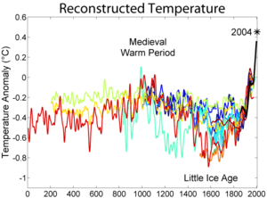
Proxies can be combined to produce temperature reconstructions longer than the instrumental temperature record and can inform discussions of global warming. The distribution of proxy records, just like the instrumental record, is not at all uniform, with more records in the northern hemisphere.[4]
Proxies
In science, it is sometimes necessary to study a variable which cannot be measured directly. This can be done by "proxy methods," in which a variable which correlates with the variable of interest is measured, and then used to infer the value of the variable of interest. Proxy methods are of particular use in the study of the past climate, beyond times when direct measurements of temperatures are available.
Most proxy records have to be calibrated against independent temperature measurements, or against a directly calibrated proxy, during their period of overlap to estimate the relationship between temperature and the proxy. The longer history of the proxy is then used to reconstruct temperature from earlier periods.
Ice cores
Drilling

Ice cores are cylindrical samples from within ice sheets in the Greenland, Antarctic, and North American regions.[5][6] First attempts of extraction occurred in 1956 as part of the International Geophysical Year. As original means of extraction, the U.S. Army’s Cold Regions Research and Engineering Laboratory used an 80-foot (24 m)-long modified electrodrill in 1968 at Camp Century, Greenland, and Byrd Station, Antarctica. Their machinery could drill through 15–20 feet of ice in 40–50 minutes. From 1300 to 3,000 feet (910 m) in depth, core samples were 4 ¼ inches in diameter and 10 to 20 feet (6.1 m) long. Deeper samples of 15 to 20 feet (6.1 m) long were not uncommon. Every subsequent drilling team improves their method with each new effort.[7]
Proxy

Presence of water molecule isotopic compositions of 16O and 18O in an ice core help determine past temperatures and snow accumulations.[5] The heavier isotope (18O) condenses more readily as temperatures decrease and falls as precipitation, while the lighter isotope (16O) can fall in even colder conditions. The farther north elevated levels of an 18O isotope are detected signals a warming over time.[8]
In addition to oxygen isotopes, water contains hydrogen isotopes - 1H and 2H, usually referred to as H and D (for deuterium) - that are also used for temperature proxies. Normally, ice cores from Greenland are analyzed for δ18O and those from Antarctica for δ-deuterium. Those cores that analyze for both show a lack of agreement. (In the figure, δ18O is for the trapped air, not the ice. δD is for the ice.)
Air bubbles in the ice, which contain trapped greenhouse gases such as carbon dioxide and methane, are also helpful in determining past climate changes.[5]
From 1989-1992, the European Greenland Ice Core Drilling Project drilled in central Greenland at coordinates 72° 35' N, 37° 38' W. In their project, ice at a depth of 770 m were 3840 years old; 2521 m were 40,000 years old; and 3029 m at bedrock were 200,000 years old or more.[9] However, ice cores can reveal the climate records for the past 650,000 years.[5]
Location maps and a complete list of U.S. ice core drilling sites can be found on the website for the National Ice Core Laboratory: http://nicl.usgs.gov/coresite.htm[6]
Tree rings

Dendroclimatology is the science of determining past climates from trees, primarily from properties of the annual tree rings. Tree rings are wider when conditions favor growth, narrower when times are difficult. Other properties of the annual rings, such as maximum latewood density (MXD) have been shown to be better proxies than simple ring width. Using tree rings, scientists have estimated many local climates for hundreds to thousands of years previous. By combining multiple tree-ring studies (sometimes with other climate proxy records), scientists have estimated past regional and global climates (see Temperature record of the past 1000 years).
Fossil leaves
New approaches retrieve data such as CO2 content of past atmospheres from fossil leaf stomata and isotope composition, measuring cellular CO2 concentrations. A 2014 study was able to use the carbon-13 isotope ratios to estimate the CO2 amounts of the past 400 million years, the findings hint at a higher climate sensitivity to CO2 concentrations.[10]
Boreholes
Borehole temperatures are used as temperature proxies. Since heat transfer through the ground is slow, temperature measurements at a series of different depths down the borehole, adjusted for the effect of rising heat from inside the Earth, can be "inverted" (a mathematical formula to solve matrix equations) to produce a non-unique series of surface temperature values. The solution is "non-unique" because there are multiple possible surface temperature reconstructions that can produce the same borehole temperature profile. In addition, due to physical limitations, the reconstructions are inevitably "smeared", and become more smeared further back in time. When reconstructing temperatures around 1,500 AD, boreholes have a temporal resolution of a few centuries. At the start of the 20th Century, their resolution is a few decades; hence they do not provide a useful check on the instrumental temperature record.[11][12] However, they are broadly comparable.[4] These confirmations have given paleoclimatologists the confidence that they can measure the temperature of 500 years ago. This is concluded by a depth scale of about 492 feet (150 meters) to measure the temperatures from 100 years ago and 1,640 feet (500 meters) to measure the temperatures from 1,000 years ago.[13]
Boreholes have a great advantage over many other proxies in that no calibration is required: they are actual temperatures. However, they record surface temperature not the near-surface temperature (1.5 meter) used for most "surface" weather observations. These can differ substantially under extreme conditions or when there is surface snow. In practice the effect on borehole temperature is believed to be generally small. A second source of error is contamination of the well by groundwater may affect the temperatures, since the water "carries" more modern temperatures with it. This effect is believed to be generally small, and more applicable at very humid sites.[11] It does not apply in ice cores where the site remains frozen all year.
More than 600 boreholes, on all continents, have been used as proxies for reconstructing surface temperatures.[12] The highest concentration of boreholes exist in North America and Europe. Their depths of drilling typically range from 200 to greater than 1,000 meters into the crust of the Earth or ice sheet.[13]
A small number of boreholes have been drilled in the ice sheets; the purity of the ice there permits longer reconstructions. Central Greenland borehole temperatures show "a warming over the last 150 years of approximately 1°C ± 0.2°C preceded by a few centuries of cool conditions. Preceding this was a warm period centered around A.D. 1000, which was warmer than the late 20th century by approximately 1°C." A borehole in the Antarctica icecap shows that the "temperature at A.D. 1 [was] approximately 1°C warmer than the late 20th century".[14]
Borehole temperatures in Greenland were responsible for an important revision to the isotopic temperature reconstruction, revealing that the former assumption that "spatial slope equals temporal slope" was incorrect.
Corals
Ocean coral skeletal rings, or bands, also share paleoclimatological information, similarly to tree rings. In 2002, a report was published on the findings of Drs. Lisa Greer and Peter Swart, associates of University of Miami at the time, in regard to stable oxygen isotopes in the calcium carbonate of coral. Cooler temperatures tend to cause coral to use heavier isotopes in its structure, while warmer temperatures result in more normal oxygen isotopes being built into the coral structure. Denser water salinity also tends to contain the heavier isotope. Greer’s coral sample from the Atlantic Ocean was taken in 1994 and dated back to 1935. Greer recalls her conclusions, "When we look at the averaged annual data from 1935 to about 1994, we see it has the shape of a sine wave. It is periodic and has a significant pattern of oxygen isotope composition that has a peak at about every twelve to fifteen years." Surface water temperatures have coincided by also peaking every twelve and a half years. However, since recording this temperature has only been practiced for the last fifty years, correlation between recorded water temperature and coral structure can only be drawn so far back.[15]
Pollen grains
Pollen can be found in sediments. Plants produce pollen in large quantities and it is extremely resistant to decay. It is possible to identify a plant species from its pollen grain. The identified plant community of the area at the relative time from that sediment layer, will provide information about the climatic condition. The abundance of pollen of a given vegetation period or year depends partly on the weather conditions of the previous months, hence pollen density provides information on short-term climatic conditions.[16] The study of prehistoric pollen is palynology.
Lake and ocean sediments
Similar to their study on other proxies, paleoclimatologists examine oxygen isotopes in the contents of ocean sediments. Likewise, they measure the layers of varve (deposited fine and coarse silt or clay)[17] laminating lake sediments. Lake varves are primarily influenced by:
- Summer temperature, which shows the energy available to melt seasonal snow and ice
- Winter snowfall, which determines the level of disturbance to sediments when melting occurs
- Rainfall[18]
Diatons and forams are also used as proxies for ocean temperatures and conditions. The oxygen isotope ratios in their shells are used as proxies for temperature. Also warmer conditions have more of them in the sediment. Also the distribution of the species of these and other sea creatures preserved in the sediments are useful proxies, for the optimal conditions for the most numerous species in the sediment. [19]
Water isotopes and temperature reconstruction
Ocean water is mostly H216O, with small amounts of HD16O and H218O, where D denotes deuterium, i.e. hydrogen with an extra neutron. In Vienna Standard Mean Ocean Water (VSMOW) the ratio of D to H is 155.76x10⁻⁶ and O-18 to O-16 is 2005.2x10−6. Isotope fractionation occurs during changes between condensed and vapour phases: the vapour pressure of heavier isotopes is lower, so vapour contains relatively more of the lighter isotopes and when the vapour condenses the precipitation preferentially contains heavier isotopes. The difference from VSMOW is expressed as δ18O = 1000‰ ; and a similar formula for δD. δ values for precipitation are always negative.[20] The major influence on δ is the difference between ocean temperatures where the moisture evaporated and the place where the final precipitation occurred; since ocean temperatures are relatively stable the δ value mostly reflects the temperature where precipitation occurs. Taking into account that the precipitation forms above the inversion layer, we are left with a linear relation:
![{\textstyle \times \left( \frac{([{}^{18}O]/[{}^{16}O])}{([{}^{18}O]/[{}^{16}O])_{\mathrm{VSMOW}}} - 1\right)}](../I/m/88021f784efed1a279b3c9c152f3bd1f3462723d.svg)
δ 18O = aT + b
This is empirically calibrated from measurements of temperature and δ as a = 0.67 ‰/°C for Greenland and 0.76 ‰/°C for East Antarctica. The calibration was initially done on the basis of spatial variations in temperature and it was assumed that this corresponded to temporal variations.[21] More recently, borehole thermometry has shown that for glacial-interglacial variations, a = 0.33 ‰/°C,[22] implying that glacial-interglacial temperature changes were twice as large as previously believed.
Pseudoproxies
The skill of algorithms used to combine proxy records into an overall hemispheric temperature reconstruction may be tested using a technique known as "pseudoproxies". In this method, output from a climate model is sampled at locations corresponding to the known proxy network, and the temperature record produced is compared to the (known) overall temperature of the model.[23]
See also
- Paleothermometer
- Ice core
- Dendrochronology
- Historical climatology, the study of climate over human history (as opposed to the earth's)
- Palynology
- Speleothem
References
- ↑ Bruckner, Monica. "Paleoclimatology: How Can We Infer Past Climates?"
- ↑ Strom, Robert G. (2007). Hot house: global climate change and the human condition. Copernicus Books. p. 253. ISBN 978-0-387-34179-8.
- ↑ "Climate Change 2001: 2.3.2.1 Palaeoclimate proxy indicators."
- 1 2 "Borehole Temperatures Confirm Global Warming Pattern."
- 1 2 3 4 Strom, Robert. Hot House. p. 255
- 1 2 "Core Location Maps."
- ↑ Vardiman, Larry, Ph.D. Ice Cores and the Age of the Earth. p. 9-13
- ↑ "Paleoclimatology: the Oxygen Balance."
- ↑ "The GRIP Coring Effort."
- ↑ Peter J. Franks, Dana L. Royer, David J. Beerling, Peter K. Van de Water, David J. Cantrill, Margaret M. Barbour and Joseph A. Berry (16 July 2014). "New constraints on atmospheric CO2 concentration for the Phanerozoic" (PDF). Geophysical Research Letters. 31 (13). doi:10.1002/2014GL060457.
- 1 2 http://www.nap.edu/openbook.php?record_id=11676&page=80
- 1 2 Pollack, H. N.; Huang, S.; Shen, P. Y. (2000). "Temperature trends over the past five centuries reconstructed from borehole temperatures". Nature. 403 (6771): 756–758. doi:10.1038/35001556.
- 1 2 Environmental News Network staff. "Borehole temperatures confirm global warming."
- ↑ BOREHOLES IN GLACIAL ICE Surface Temperature Reconstructions for the Last 2,000 Years (2006), pp 81,82 Board on Atmospheric Sciences and Climate (BASC), National Academy of Science, ISBN 978-0-309-10225-4
- ↑ "Coral Layers Good Proxy for Atlantic Climate Cycles."
- ↑ Bradley, R. S. and Jones, P. D. (eds) 1992: Climate since AD 1500. London: Routledge.
- ↑ "Varve."
- ↑ "Climate Change 2001: 2.3.2.1 Palaeoclimate proxy indicators"
- ↑ Bruckner, Monica. "Paleoclimatology: How Can We Infer Past Climates?". Montana State University.
- ↑ http://books.nap.edu/openbook.php?record_id=11676&page=66
- ↑ Jouzel and Merlivat, 1984) Deuterium and oxygen 18 in precipitation: Modeling of the isotopic effects during snow formation, Journal of Geophysical Research: Atmospheres, Volume 89, Issue D7, Pages 11589–11829
- ↑ Cuffey et al., 1995, Large Arctic temperature change at the Wisconsin– Holocene glacial transition, Science 270: 455–458
- ↑ Mann, M. E.; Rutherford, S. (31 May 2002), "Climate reconstruction using 'Pseudoproxies'", Geophysical Research Letters, 29 (10), doi:10.1029/2001GL014554
- Sources
- "Borehole Temperatures Confirm Global Warming Pattern." UniSci. 27 Feb. 2001. 7 Oct. 2009.
- Bruckner, Monica. "Paleoclimatology: How Can We Infer Past Climates?" Microbial Life. 29 Sept. 2008. 23 Nov. 2009.
- "Climate Change 2001: 2.3.2.1 Palaeoclimate proxy indicators." IPCC. 2003. Sept. 23, 2009.
- "Coral Layers Good Proxy for Atlantic Climate Cycles." Earth Observatory. Webmaster: Paul Przyborski. 7 Dec. 2002. 2 Nov. 2009.
- "Core Location Maps." National Ice Core Laboratory. 9 Apr. 2009. 23 Nov. 2009.
- "Dendrochronology." Merriam-Webster Online Dictionary. Merriam-Webster Online. 2009. 2 Oct. 2009.
- Environmental News Network staff. "Borehole temperatures confirm global warming." CNN.com. 17 Feb. 2000. 7 Oct. 2009.
- "The GRIP Coring Effort." NCDC. 26 Sept. 2009.
- "Growth ring." Encyclopædia Britannica. Encyclopædia Britannica Online. 2009. 23 Oct. 2009.
- Huang, Shaopeng, et al. "Temperature trends over the past five centuries reconstructed from borehole temperatures." Nature. 2009. 6 Oct. 2009.
- "Objectives - Kola Superdeep Borehole (KSDB) - IGCP 408: ‘Rocks and Minerals at Great Depths and on the Surface.’" International Continental Scientific Drilling Program. 18 July 2006. 6 Oct. 2009.
- "Paleoclimatology: the Oxygen Balance." Earth Observatory. Webmaster: Paul Przyborski. 24 Nov. 2009. 24 Nov. 2009.
- Schweingruber, Fritz Hans. Tree Rings: Basics and Application of Dendrochronology. Dordrecht: 1988. 2, 47-8, 54, 256-7.
- Strom, Robert. Hot House. New York: Praxis, 2007. 255.
- "Varve." Merriam-Webster Online Dictionary. Merriam-Webster Online. 2009. 2 Nov. 2009.
- Wolff, E. W. (2000) History of the atmosphere from ice cores; ERCA vol 4 pp 147–177
External links
- Chemical climate proxies at Royal Society of Chemistry, January 23, 2013