Nomogram

A nomogram (from Greek νόμος nomos, "law" and γραμμή grammē, "line"), also called a nomograph, alignment chart or abaque, is a graphical calculating device, a two-dimensional diagram designed to allow the approximate graphical computation of a mathematical function. The field of nomography was invented in 1884 by the French engineer Philbert Maurice d’Ocagne (1862-1938) and used extensively for many years to provide engineers with fast graphical calculations of complicated formulas to a practical precision. Nomograms use a parallel coordinate system invented by d'Ocagne rather than standard Cartesian coordinates.
A nomogram consists of a set of n scales, one for each variable in an equation. Knowing the values of n-1 variables, the value of the unknown variable can be found, or by fixing the values of some variables, the relationship between the unfixed ones can be studied. The result is obtained by laying a straightedge across the known values on the scales and reading the unknown value from where it crosses the scale for that variable. The virtual or drawn line created by the straightedge is called an index line or isopleth.
Nomograms flourished in many different contexts for roughly 75 years because they allowed quick and accurate computations before the age of pocket calculators. Results from a nomogram are obtained very quickly and reliably by simply drawing one or more lines. The user does not have to know how to solve algebraic equations, look up data in tables, use a slide rule, or substitute numbers into equations to obtain results. The user does not even need to know the underlying equation the nomogram represents. In addition, nomograms naturally incorporate implicit or explicit domain knowledge into their design. For example, to create larger nomograms for greater accuracy the nomographer usually includes only scale ranges that are reasonable and of interest to the problem. Many nomograms include other useful markings such as reference labels and colored regions. All of these provide useful guideposts to the user.
Like a slide rule, a nomogram is a graphical analog computation device, and like the slide rule, its accuracy is limited by the precision with which physical markings can be drawn, reproduced, viewed, and aligned. While the slide rule is intended to be a general-purpose device, a nomogram is designed to perform a specific calculation, with tables of values effectively built into the construction of the scales. Nomograms are typically used in applications where the level of accuracy they offer is sufficient and useful. Alternatively, a nomogram can be used to check an answer obtained from another, more exact but possibly error-prone calculation.
Other types of graphical calculators such as intercept charts, trilinear diagrams and hexagonal charts are sometimes called nomograms. Other such examples include the Smith chart, a graphical calculator used in electronics and systems analysis, thermodynamic diagrams and tephigrams, used to plot the vertical structure of the atmosphere and perform calculations on its stability and humidity content. These do not meet the strict definition of a nomogram as a graphical calculator whose solution is found by the use of one or more linear isopleths.
Description

A nomogram for a three-variable equation typically has three scales, although there exist nomograms in which two or even all three scales are common. Here two scales represent known values and the third is the scale where the result is read off. The simplest such equation is u1 + u2 + u3 = 0 for the three variables u1, u2 and u3. An example of this type of nomogram is shown on the right, annotated with terms used to describe the parts of a nomogram.
More complicated equations can sometimes be expressed as the sum of functions of the three variables. For example, the nomogram at the top of this article could be constructed as a parallel-scale nomogram because it can be expressed as such a sum after taking logarithms of both sides of the equation.
The scale for the unknown variable can lie between the other two scales or outside of them. The known values of the calculation are marked on the scales for those variables, and a line is drawn between these marks. The result is read off the unknown scale at the point where the line intersects that scale. The scales include 'tick marks' to indicate exact number locations, and they may also include labeled reference values. These scales may be linear, logarithmic, or have some more complex relationship.
The sample isopleth shown in red on the nomogram at the top of this article calculates the value of T when S = 7.30 and R = 1.17. The isopleth crosses the scale for T at just under 4.65; a larger figure printed in high resolution on paper would yield T = 4.64 to three-digit precision. Note that any variable can be calculated from values of the other two, a feature of nomograms that is particularly useful for equations in which a variable cannot be algebraically isolated from the other variables.
Straight scales are useful for relatively simple calculations, but for more complex calculations the use of simple or elaborate curved scales may be required. Nomograms for more than three variables can be constructed by incorporating a grid of scales for two of the variables, or by concatenating individual nomograms of fewer numbers of variables into a compound nomogram.
Applications
Nomograms have been used in an extensive array of applications. A sample includes
- The original application by d'Ocagne, the automation of complicated cut and fill calculations for earth removal during the construction of the French national railway system. This was an important proof of concept, because the calculations are non-trivial and the results translated into significant savings of time, effort, and money.
- The design of channels, pipes and weirs for regulating the flow of water.
- The work of Lawrence Henderson, in which nomograms were used to correlate many different aspects of blood physiology. It was the first major use of nomograms in the United States and also the first medical nomograms anywhere. Nomograms continue to be used extensively in medical fields.
- Ballistics calculations prior to fire control systems, where calculating time was critical.
- Machine shop calculations, to convert blueprint dimensions and perform calculations based on material dimensions and properties. These nomograms often included markings for standard dimensions and for available manufactured parts.
- Statistics, for complicated calculations of properties of distributions and for operations research including the design of acceptance tests for quality control.
- Operations Research, to obtain results in a variety of optimization problems.
- Chemistry and chemical engineering, to encapsulate both general physical relationships and empirical data for specific compounds.
- Aeronautics, in which nomograms were used for decades in the cockpits of aircraft of all descriptions. As a navigation and flight control aid, nomograms were fast, compact and easy-to-use calculators.
- Astronomical calculations, as in the post-launch orbital calculations of Sputnik 1 by P.E. Elyasberg.[1]
- Engineering work of all kinds: Electrical design of filters and transmission lines, mechanical calculations of stress and loading, optical calculations, and so forth.
- Military, where complex calculations need to be made in the field quickly and with reliability not dependent on electrical devices.
Examples
Parallel-resistance/thin-lens

The nomogram below performs the computation

This nomogram is interesting because it performs a useful nonlinear calculation using only straight-line, equally graduated scales.
A and B are entered on the horizontal and vertical scales, and the result is read from the diagonal scale. Being proportional to the harmonic mean of A and B, this formula has several applications. For example, it is the parallel-resistance formula in electronics, and the thin-lens equation in optics.
In the example, the red line demonstrates that parallel resistors of 56 and 42 ohms have a combined resistance of 24 ohms. It also demonstrates that an object at a distance of 56 cm from a lens whose focal length is 24 cm forms a real image at a distance of 42 cm.
Chi-squared test computation

The nomogram below can be used to perform an approximate computation of some values needed when performing a familiar statistical test, Pearson's chi-squared test. This nomogram demonstrates the use of curved scales with unevenly spaced graduations.
The relevant expression is
The scale along the top is shared among five different ranges of observed values: A, B, C, D and E. The observed value is found in one of these ranges, and the tick mark used on that scale is found immediately above it. Then the curved scale used for the expected value is selected based on the range. For example, an observed value of 9 would use the tick mark above the 9 in range A, and curved scale A would be used for the expected value. An observed value of 81 would use the tick mark above 81 in range E, and curved scale E would be used for the expected value. This allows five different nomograms to be incorporated into a single diagram.
In this manner, the blue line demonstrates the computation of
- (9 − 5)2/ 5 = 3.2
and the red line demonstrates the computation of
- (81 − 70)2 / 70 = 1.7
In performing the test, Yates's correction for continuity is often applied, and simply involves subtracting 0.5 from the observed values. A nomogram for performing the test with Yates's correction could be constructed simply by shifting each "observed" scale half a unit to the left, so that the 1.0, 2.0, 3.0, ... graduations are placed where the values 0.5, 1.5, 2.5, ... appear on the present chart.
Food risk assessment
.png)
Although nomograms represent mathematical relationships, not all are mathematically derived. The following one was developed graphically to achieve appropriate end results that could readily be defined by the product of their relationships in subjective units rather than numerically. The use of non-parallel axes enabled the non-linear relationships to be incorporated into the model.
The numbers in square boxes denote the axes requiring input after appropriate assessment.
The pair of nomograms at the top of the image determine the probability of occurrence and the availability, which are then incorporated into the bottom multistage nomogram.
Lines 8 and 10 are ‘tie lines’ or ‘pivot lines’ and are used for the transition between the stages of the compound nomogram.
The final pair of parallel logarithmic scales (12) are not nomograms as such, but reading-off scales to translate the risk score (11, remote to extremely high) into a sampling frequency to address safety aspects and other ‘consumer protection’ aspects respectively. This stage requires political ‘buy in’ balancing cost against risk. The example uses a three-year minimum frequency for each, though with the high risk end of the scales different for the two aspects, giving different frequencies for the two, but both subject to an overall minimum sampling of every food for all aspects at least once every three years.
This risk assessment nomogram was developed by the UK Public Analyst Service with funding from the UK Food Standards Agency for use as a tool to guide the appropriate frequency of sampling and analysis of food for official food control purposes, intended to be used to assess all potential problems with all foods, although not yet adopted.
Sample size estimation
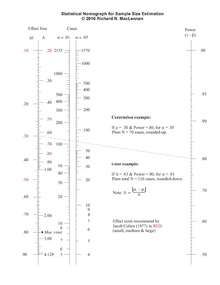
This nomograph can be used to estimate the sample size requirements for statistical analyses. It uses four parameters (one of which is fixed): effect size (rho or delta), statistical power, alpha (fixed), and number of cases.
The hypothesized effect size in the population can either be expressed as a correlation coefficient (rho) or a standardized difference in means (delta) for a t-test. The standardized difference is equal to the absolute value of the difference between two population means (mu's), divided by the pooled population standard deviation (sigma).
The statistical power desired is estimated by one minus beta, where beta is equal to the probability of making a Type II error. A Type II error is failing to reject that statistical null hypothesis (i.e., rho or delta equals zero), when in fact the null hypothesis is false in the population and should be rejected. Cohen (1977) recommends using power equal to .80 or 80%, for a beta = .20.
The sample size or number of cases required is reported for two fixed levels of statistical significance (alpha = .01 or .05). Alpha is the probability of making a Type I error. A Type I error is rejecting the statistical null hypothesis (i.e., rho or delta equals zero), when in fact it is true in the population and should not be rejected. The most commonly used values of alpha are .05 or .01.
To find the sample size requirements for a given statistical analysis, estimate the effect size expected in the population (rho or delta) on the left hand axis, select the desired level of power on the right hand axis, and draw a line between the two values.
Where the line intersects with either the alpha = .05 or alpha = .01 middle axis will indicate the sample size required to achieve statistical significance of alpha less than .05 or .01, respectively (for the previously given parameters).
For instance, if one estimates the population correlation (rho) to be .30, and desires statistical power equal to .80, then to obtain a significance level of alpha less than .05, the sample size requirement would be N = 70 cases rounded up (more precisely approximately 68 cases using interpolation).
Cohen, J. (1977). Statistical power analysis for the behavioral sciences. 2nd. ed. San Diego, CA: Academic Press
See also
References
- ↑ Yu.A.Mozzhorin Memories at the website of Russian state archive for scientific-technical documentation
- D.P. Adams, Nomography: Theory and Application, (Archon Books) 1964.
- H.J. Allcock, J. Reginald Jones, and J.G.L. Michel, The Nomogram. The Theory and Practical Construction of Computation Charts, 5th ed., (London: Sir Isaac Pitman & Sons, Ltd.) 1963.
- S. Brodestsky, A First Course in Nomography, (London, G. Bell and Sons) 1920.
- D.S. Davis, Empirical Equations and Nomography, (New York: McGraw-Hill Book Co.) 1943.
- M. d'Ocagne: Traité de Nomographie, (Gauthier-Villars, Paris) 1899.
- M. d'Ocagne: (1900) Sur la résolution nomographique de l'équation du septième degré. Comptes rendus (Paris), 131, 522–524.
- R.D. Douglass and D.P. Adams, Elements of Nomography, (New York: McGraw-Hill) 1947.
- R.P. Hoelscher, et al., Graphic Aids in Engineering Computation, (New York: McGraw-Hill) 1952.
- L. Ivan Epstein, Nomography, (New York: Interscience Publishers) 1958.
- L.H. Johnson, Nomography and Empirical Equations, (New York: John Wiley and Sons) 1952.
- M. Kattan and J. Marasco. (2010) What Is a Real Nomogram?, Seminars in oncology, 37(1), 23–26.
- A.S. Levens, Nomography, 2nd ed., (New York: John Wiley & Sons, Inc.) 1959.
- F.T. Mavis, The Construction of Nomographic Charts, (Scranton, International Textbook) 1939.
- E. Otto, Nomography,(New York: The Macmillan Company) 1963.
- H.A. Evesham The History and Development of Nomography, (Boston: Docent Press) 2010. ISBN 9781456479626
- T.H. Gronwall, R. Doerfler, A. Gluchoff, and S. Guthery, Calculating Curves: The Mathematics, History, and Aesthetic Appeal of T. H. Gronwall's Nomographic Work, (Boston: Docent Press) 2012. ISBN 9780983700432
External links
| Wikimedia Commons has media related to Nomograms. |
| Look up nomogram in Wiktionary, the free dictionary. |
- The Art of Nomography describes the design of nomograms using geometry, determinants, and transformations.
- The Lost Art of Nomography is a math journal article surveying the field of nomography.
- Nomograms for Wargames but also of general interest.
- PyNomo – open source software for constructing nomograms.
- Java Applet for constructing simple nomograms.
- Nomograms for visualising relationships between three variables - video and slides of invited talk by Jonathan Rougier for useR!2011.