Rectangle method
In mathematics, specifically in integral calculus, the rectangle method (also called the midpoint or mid-ordinate rule) computes an approximation to a definite integral, made by finding the area of a collection of rectangles whose heights are determined by the values of the function.
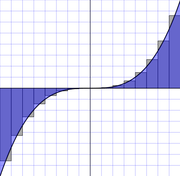
Specifically, the interval over which the function is to be integrated is divided into equal subintervals of length . The rectangles are then drawn so that either their left or right corners, or the middle of their top line lies on the graph of the function, with bases running along the -axis. The approximation to the integral is then calculated by adding up the areas (base multiplied by height) of the rectangles, giving the formula:


where and .

The formula for above gives for the Top-left corner approximation.

As N gets larger, this approximation gets more accurate. In fact, this computation is the spirit of the definition of the Riemann integral and the limit of this approximation as is defined and equal to the integral of on if this Riemann integral is defined. Note that this is true regardless of which is used, however the midpoint approximation tends to be more accurate for finite .


| The different rectangle approximations | ||
|---|---|---|
|
Error
For a function which is twice differentiable, the approximation error in each section of the midpoint rule decays as the cube of the width of the rectangle. (For a derivation based on a Taylor approximation, see Midpoint method)


for some in . Summing this, the approximation error for intervals with width is less than or equal to


where is the number of nodes


in terms of the total interval, we know that so we can rewrite the expression:


which is equal to:

for some in .