Methods of computing square roots

The sequence we get by computing the square root of two with the Babylonian method with different starting points

In numerical analysis, a branch of mathematics, there are several square root algorithms or methods of computing the principal square root of a non-negative real number. For the square roots of a negative or complex number, see below.

Finding ${\sqrt {S}}$ is the same as solving the equation $f(x)=x^{2}-S=0\,\!$ for a positive $x$ . Therefore, any general numerical root-finding algorithm can be used. Newton's method, for example, reduces in this case to the so-called Babylonian method:

x_{n+1}=x_{n}-{\frac {f(x_{n})}{f'(x_{n})}}=x_{n}-{\frac {x_{n}^{2}-S}{2x_{n}}}={\frac {1}{2}}\left(x_{n}+{\frac {S}{x_{n}}}\right)

These methods generally yield approximate results, but can be made arbitrarily precise by increasing the number of calculation steps.

Rough estimation

Many square root algorithms require an initial seed value. If the initial seed value is far away from the actual square root, the algorithm will be slowed down. It is therefore useful to have a rough estimate, which may be very inaccurate but easy to calculate. With $S$ expressed in scientific notation as $a\times 10^{2n}$ where $1\leq a<100$ and n is an integer, the square root ${\sqrt {S}}={\sqrt {a}}\times 10^{n}$ can be estimated as

{\sqrt {S}}\approx {\begin{cases}2\cdot 10^{n}&{\text{if }}a<10,\\6\cdot 10^{n}&{\text{if }}a\geq 10.\end{cases}}

The factors two and six are used because they approximate the geometric means of the lowest and highest possible values with the given number of digits: ${\sqrt {{\sqrt {1}}\cdot {\sqrt {10}}}}={\sqrt[{4}]{10}}\approx 2\,$ and ${\sqrt {{\sqrt {10}}\cdot {\sqrt {100}}}}={\sqrt[{4}]{1000}}\approx 6\,$ .

For $S=125348=12.5348\times 10^{4}$ , the estimate is ${\sqrt {S}}\approx 6\cdot 10^{2}=600$ .

When working in the binary numeral system (as computers do internally), by expressing $S$ as $a\times 2^{2n}$ where $0.1_{2}\leq a<10_{2}$ , the square root ${\sqrt {S}}={\sqrt {a}}\times 2^{n}$ can be estimated as ${\sqrt {S}}\approx 2^{n}$ , since the geometric mean of the lowest and highest possible values is ${\sqrt {{\sqrt {0.1_{2}}}\cdot {\sqrt {10_{2}}}}}={\sqrt[{4}]{1}}=1$ .

For $S=125348=1\;1110\;1001\;1010\;0100_{2}=1.1110\;1001\;1010\;0100_{2}\times 2^{16}\,$ the binary approximation gives ${\sqrt {S}}\approx 2^{8}=1\;0000\;0000_{2}=256\,.$

These approximations are useful to find better seeds for iterative algorithms, which results in faster convergence.

Babylonian method

"Heron's method" redirects here. For the formula used to find the area of a triangle, see Heron's formula.

Graph charting the use of the Babylonian method for approximating the square root of 100 (10) using starting values x₀ = 50, x₀ = 1, and x₀ = −5. Note that using a negative starting value yields the negative root.

Perhaps the first algorithm used for approximating $\sqrt S$ is known as the Babylonian method, named after the Babylonians,^[1] or "Hero's method", named after the first-century Greek mathematician Hero of Alexandria who gave the first explicit description of the method.^[2] It can be derived from (but predates by 16 centuries) Newton's method. The basic idea is that if $x$ is an overestimate to the square root of a non-negative real number $S$ then $S / x$ will be an underestimate and so the average of these two numbers may reasonably be expected to provide a better approximation (though the formal proof of that assertion depends on the inequality of arithmetic and geometric means that shows this average is always an overestimate of the square root, as noted in the article on square roots, thus assuring convergence).

More precisely, if $x$ is our initial guess of $\sqrt S$ and $e$ is the error in our estimate such that $S = (x + e) 2$ , then we can expand the binomial and solve for

e={\frac {S-x^{2}}{2x+e}}\approx {\frac {S-x^{2}}{2x}},

since

e\ll x

Therefore, we can compensate for the error and update our old estimate as

x:=x+e={\frac {S+x^{2}}{2x}}={\frac {x+{\frac {S}{x}}}{2}}

Since the computed error was not exact, this becomes our next best guess. The process of updating is iterated until desired accuracy is obtained. This is a quadratically convergent algorithm, which means that the number of correct digits of the approximation roughly doubles with each iteration. It proceeds as follows:

Begin with an arbitrary positive starting value $x 0$ (the closer to the actual square root of $S$ , the better).
Let $x n + 1$ be the average of $x n$ and $S / x n$ (using the arithmetic mean to approximate the geometric mean).
Repeat step 2 until the desired accuracy is achieved.

It can also be represented as:

x_{0}\approx {\sqrt {S}},

x_{n+1}={\frac {1}{2}}\left(x_{n}+{\frac {S}{x_{n}}}\right),

{\sqrt {S}}=\lim _{n\to \infty }x_{n}.

This algorithm works equally well in the $p$ -adic numbers, but cannot be used to identify real square roots with $p$ -adic square roots; one can, for example, construct a sequence of rational numbers by this method that converges to +3 in the reals, but to −3 in the 2-adics.

Example

To calculate $\sqrt S$ , where $S$ = 125348, to six significant figures, use the rough estimation method above to get

{\begin{aligned}{\begin{array}{rlll}x_{0}&=6\cdot 10^{2}&&=600.000\\[0.3em]x_{1}&={\frac {1}{2}}\left(x_{0}+{\frac {S}{x_{0}}}\right)&={\frac {1}{2}}\left(600.000+{\frac {125348}{600.000}}\right)&=404.457\\[0.3em]x_{2}&={\frac {1}{2}}\left(x_{1}+{\frac {S}{x_{1}}}\right)&={\frac {1}{2}}\left(404.457+{\frac {125348}{404.457}}\right)&=357.187\\[0.3em]x_{3}&={\frac {1}{2}}\left(x_{2}+{\frac {S}{x_{2}}}\right)&={\frac {1}{2}}\left(357.187+{\frac {125348}{357.187}}\right)&=354.059\\[0.3em]x_{4}&={\frac {1}{2}}\left(x_{3}+{\frac {S}{x_{3}}}\right)&={\frac {1}{2}}\left(354.059+{\frac {125348}{354.059}}\right)&=354.045\\[0.3em]x_{5}&={\frac {1}{2}}\left(x_{4}+{\frac {S}{x_{4}}}\right)&={\frac {1}{2}}\left(354.045+{\frac {125348}{354.045}}\right)&=354.045\end{array}}\end{aligned}}

Therefore, $\sqrt 125348 \approx 354.045$ .

Convergence

Let the relative error in $x n$ be defined by

\varepsilon _{n}={\frac {x_{n}}{\sqrt {S}}}-1

and thus

x_{n}={\sqrt {S}}\cdot (1+\varepsilon _{n}).

Then it can be shown that

\varepsilon _{n+1}={\frac {\varepsilon _{n}^{2}}{2(1+\varepsilon _{n})}}

and thus that

0\leq \varepsilon _{n+2}\leq \min \left\{{\frac {\varepsilon _{n+1}^{2}}{2}},{\frac {\varepsilon _{n+1}}{2}}\right\}

and consequently that convergence is assured provided that $x 0$ and $S$ are both positive.

Worst case for convergence

If using the rough estimate above with the Babylonian method, then the least accurate cases in ascending order are as follows:

{\begin{aligned}S&=1;&x_{0}&=2;&x_{1}&=1.250;&\varepsilon _{1}&=0.250.\\S&=10;&x_{0}&=2;&x_{1}&=3.500;&\varepsilon _{1}&<0.107.\\S&=10;&x_{0}&=6;&x_{1}&=3.833;&\varepsilon _{1}&<0.213.\\S&=100;&x_{0}&=6;&x_{1}&=11.333;&\varepsilon _{1}&<0.134.\end{aligned}}

Thus in any case,

\varepsilon _{1}\leq 2^{-2}.\,

\varepsilon _{2}<2^{-5}<10^{-1}.\,

\varepsilon _{3}<2^{-11}<10^{-3}.\,

\varepsilon _{4}<2^{-23}<10^{-6}.\,

\varepsilon _{5}<2^{-47}<10^{-14}.\,

\varepsilon _{6}<2^{-95}<10^{-28}.\,

\varepsilon _{7}<2^{-191}<10^{-57}.\,

\varepsilon _{8}<2^{-383}<10^{-115}.\,

Rounding errors will slow the convergence. It is recommended to keep at least one extra digit beyond the desired accuracy of the $x n$ being calculated to minimize round off error.

Digit-by-digit calculation

This is a method to find each digit of the square root in a sequence. It is slower than the Babylonian method (if you have a calculator that can divide in one operation), but it has several advantages:

It can be easier for manual calculations.
Every digit of the root found is known to be correct, i.e., it does not have to be changed later.
If the square root has an expansion that terminates, the algorithm terminates after the last digit is found. Thus, it can be used to check whether a given integer is a square number.
The algorithm works for any base, and naturally, the way it proceeds depends on the base chosen.

Napier's bones include an aid for the execution of this algorithm. The shifting nth root algorithm is a generalization of this method.

Basic principle

First, let's consider the simplest possible case of finding the square root of a number Z, that is the square of a 2 digit number XY, where X is the ten's digit and Y is the unit's digit. Specifically:

Z = (10X + Y)² = 100X² + 20XY + Y²

Now using the Digit-by-Digit algorithm, we first determine the value of X. X is the largest digit such that X² is less or equal to Z from which we removed the 2 rightmost digits.

In the next iteration, we pair the digits, multiply X by 2, and place it in the tenth's place while we try to figure out what the value of Y is.

Since this is a simple case where the answer is a perfect square root XY, the algorithm stops here.

The same idea can be extended to any arbitrary square root computation next. Suppose we are able to find the square root of N by expressing it as a sum of n positive numbers such that

N=(a_{1}+a_{2}+a_{3}+\dotsb +a_{n})^{2}.

By repeatedly applying the basic identity

(x+y)^{2}=x^{2}+2xy+y^{2},

the right-hand-side term can be expanded as

{\begin{aligned}&(a_{1}+a_{2}+a_{3}+\dotsb +a_{n})^{2}\\=&\,a_{1}^{2}+2a_{1}a_{2}+a_{2}^{2}+2(a_{1}+a_{2})a_{3}+a_{3}^{2}+\dotsb +a_{n-1}^{2}+2\left(\sum _{i=1}^{n-1}a_{i}\right)a_{n}+a_{n}^{2}\\=&\,a_{1}^{2}+[2a_{1}+a_{2}]a_{2}+[2(a_{1}+a_{2})+a_{3}]a_{3}+\dotsb +\left[2\left(\sum _{i=1}^{n-1}a_{i}\right)+a_{n}\right]a_{n}.\end{aligned}}

This expression allows us to find the square root by sequentially guessing the values of $a_{i}$ s. Suppose that the numbers $a_{1},\ldots ,a_{m-1}$ have already been guessed, then the m-th term of the right-hand-side of above summation is given by $Y_{m}=[2P_{m-1}+a_{m}]a_{m},$ where $P_{m-1}=\sum _{i=1}^{m-1}a_{i}$ is the approximate square root found so far. Now each new guess $a_{m}$ should satisfy the recursion

X_{m}=X_{m-1}-Y_{m},

such that $X_{m}\geq 0$ for all $1\leq m\leq n,$ with initialization $X_{0}=N.$ When $X_{n}=0,$ the exact square root has been found; if not, then the sum of $a_{i}$ s gives a suitable approximation of the square root, with $X_{n}$ being the approximation error.

For example, in the decimal number system we have

N=(a_{1}\cdot 10^{n-1}+a_{2}\cdot 10^{n-2}+\cdots +a_{n-1}\cdot 10+a_{n})^{2},

where $10^{n-i}$ are place holders and the coefficients $a_{i}\in \{0,1,2,\ldots ,9\}$ . At any m-th stage of the square root calculation, the approximate root found so far, $P_{m-1}$ and the summation term $Y_{m}$ are given by

P_{m-1}=\sum _{i=1}^{m-1}a_{i}\cdot 10^{n-i}=10^{n-m+1}\sum _{i=1}^{m-1}a_{i}\cdot 10^{m-i-1},

Y_{m}=[2P_{m-1}+a_{m}\cdot 10^{n-m}]a_{m}\cdot 10^{n-m}=[20\sum _{i=1}^{m-1}a_{i}\cdot 10^{m-i-1}+a_{m}]a_{m}\cdot 10^{2(n-m)}.

Here since the place value of $Y_{m}$ is an even power of 10, we only need to work with the pair of most significant digits of the remaining term $X_{m-1}$ at any m-th stage. The section below codifies this procedure.

It is obvious that a similar method can be used to compute the square root in number systems other than the decimal number system. For instance, finding the digit-by-digit square root in the binary number system is quite efficient since the value of $a_{i}$ is searched from a smaller set of binary digits {0,1}. This makes the computation faster since at each stage the value of $Y_{m}$ is either $Y_{m}=0$ for $a_{m}=0$ or $Y_{m}=2P_{m-1}+1$ for $a_{m}=1$ . The fact that we have only two possible options for $a_{m}$ also makes the process of deciding the value of $a_{m}$ at m-th stage of calculation easier. This is because we only need to check if $Y_{m}\leq X_{m-1}$ for $a_{m}=1.$ If this condition is satisfied, then we take $a_{m}=1$ ; if not then $a_{m}=0.$ Also, the fact that multiplication by 2 is done by left bit-shifts helps in the computation.

Decimal (base 10)

Write the original number in decimal form. The numbers are written similar to the long division algorithm, and, as in long division, the root will be written on the line above. Now separate the digits into pairs, starting from the decimal point and going both left and right. The decimal point of the root will be above the decimal point of the square. One digit of the root will appear above each pair of digits of the square.

Beginning with the left-most pair of digits, do the following procedure for each pair:

Starting on the left, bring down the most significant (leftmost) pair of digits not yet used (if all the digits have been used, write "00") and write them to the right of the remainder from the previous step (on the first step, there will be no remainder). In other words, multiply the remainder by 100 and add the two digits. This will be the current value c.
Find p, y and x, as follows:
- Let p be the part of the root found so far, ignoring any decimal point. (For the first step, p = 0).
- Determine the greatest digit x such that $x(20p+x)\leq c$ . We will use a new variable y = x(20p + x).
  - Note: 20p + x is simply twice p, with the digit x appended to the right).
  - Note: You can find x by guessing what c/(20·p) is and doing a trial calculation of y, then adjusting x upward or downward as necessary.
- Place the digit $x$ as the next digit of the root, i.e., above the two digits of the square you just brought down. Thus the next p will be the old p times 10 plus x.
Subtract y from c to form a new remainder.
If the remainder is zero and there are no more digits to bring down, then the algorithm has terminated. Otherwise go back to step 1 for another iteration.

Examples

Find the square root of 152.2756.

          1  2. 3  4 
       /
     \/  01 52.27 56

         01                   1*1 <= 1 < 2*2                 x = 1
         01                     y = x*x = 1*1 = 1
         00 52                22*2 <= 52 < 23*3              x = 2
         00 44                  y = (20+x)*x = 22*2 = 44
            08 27             243*3 <= 827 < 244*4           x = 3
            07 29               y = (240+x)*x = 243*3 = 729
               98 56          2464*4 <= 9856 < 2465*5        x = 4
               98 56            y = (2460+x)*x = 2464*4 = 9856
               00 00          Algorithm terminates: Answer is 12.34

Find the square root of 2.

          1. 4  1  4  2
       /
     \/  02.00 00 00 00

         02                  1*1 <= 2 < 2*2                 x = 1
         01                    y = x*x = 1*1 = 1
         01 00               24*4 <= 100 < 25*5             x = 4
         00 96                 y = (20+x)*x = 24*4 = 96
            04 00            281*1 <= 400 < 282*2           x = 1
            02 81              y = (280+x)*x = 281*1 = 281
            01 19 00         2824*4 <= 11900 < 2825*5       x = 4
            01 12 96           y = (2820+x)*x = 2824*4 = 11296
               06 04 00      28282*2 <= 60400 < 28283*3     x = 2
                             The desired precision is achieved:
                             The square root of 2 is about 1.4142

Binary numeral system (base 2)

Inherent to digit-by-digit algorithms is a search and test step: find a digit, $\,e$ , when added to the right of a current solution $\,r$ , such that $\,(r+e)\cdot (r+e)\leq x$ , where $\,x$ is the value for which a root is desired. Expanding: $\,r\cdot r+2re+e\cdot e\leq x$ . The current value of $\,r\cdot r$ —or, usually, the remainder—can be incrementally updated efficiently when working in binary, as the value of $\,e$ will have a single bit set (a power of 2), and the operations needed to compute $\,2\cdot r\cdot e$ and $\,e\cdot e$ can be replaced with faster bit shift operations.

Example

Here we obtain the square root of 81, which when converted into binary gives 1010001. The numbers in the left column gives the option between that number or zero to be used for subtraction at that stage of computation. The final answer is 1001, which in decimal is 9.

              1 0 0 1
             ---------
            √ 1010001

       1      1
              1
             ---------
       101     01  
                0
              --------
       1001     100
                  0
              --------
       10001    10001
                10001
               -------
                    0

This gives rise to simple computer implementations:^[3]

short isqrt(short num) {
    short res = 0;
    short bit = 1 << 14; // The second-to-top bit is set: 1 << 30 for 32 bits
 
    // "bit" starts at the highest power of four <= the argument.
    while (bit > num)
        bit >>= 2;
        
    while (bit != 0) {
        if (num >= res + bit) {
            num -= res + bit;
            res = (res >> 1) + bit;
        }
        else
            res >>= 1;
        bit >>= 2;
    }
    return res;
}

Using the notation above, the variable "bit" corresponds to $e_{m}^{2}$ which is $(2^{m})^{2}=4^{m}$ , the variable "res" is equal to $2re_{m}$ , and the variable "num" is equal to the current $X_{m}$ which is the difference of the number we want the square root of and the square of our current approximation with all bits set up to $2^{m+1}$ . Thus in the first loop, we want to find the highest power of 4 in "bit" to find the highest power of 2 in $e$ . In the second loop, if num is greater than res + bit, then $X_{m}$ is greater than $2re_{m}+e_{m}^{2}$ and we can subtract it. The next line, we want to add $e_{m}$ to $r$ which means we want to add $2e_{m}^{2}$ to $2re_{m}$ so we want res = res + bit<<1. Then update $e_{m}$ to $e_{m-1}$ inside res which involves dividing by 2 or another shift to the right. Combining these 2 into one line leads to res = res>>1 + bit. If $X_{m}$ isn't greater than $2re_{m}+e_{m}^{2}$ then we just update $e_{m}$ to $e_{m-1}$ inside res and divide it by 2. Then we update $e_{m}$ to $e_{m-1}$ in bit by dividing it by 4. The final iteration of the 2nd loop has bit equal to 1 and will cause update of $e$ to run one extra time removing the factor of 2 from res making it our integer approximation of the root.

Faster algorithms, in binary and decimal or any other base, can be realized by using lookup tables—in effect trading more storage space for reduced run time.^[4]

Exponential identity

Pocket calculators typically implement good routines to compute the exponential function and the natural logarithm, and then compute the square root of S using the identity found using the properties of logarithms ( $\ln x^{n}=n\ln x$ ) and exponentials ( $e^{\ln x}=x$ ):

{\sqrt {S}}=e^{{\frac {1}{2}}\ln S}.

The denominator in the fraction corresponds to the nth root. In the case above the denominator is 2, hence the equation specifies that the square root is to be found. The same identity is used when computing square roots with logarithm tables or slide rules.

Bakhshali approximation

This method for finding an approximation to a square root was described in an ancient Indian mathematical manuscript called the Bakhshali manuscript. It is equivalent to two iterations of the Babylonian method beginning with N. The original presentation goes as follows: To calculate ${\sqrt {S}}$ , let N² be the nearest perfect square to S. Then, calculate:

d=S-N^{2}\,\!

P={\frac {d}{2N}}

A=N+P\,\!

{\sqrt {S}}\approx A-{\frac {P^{2}}{2A}}

This can be also written as:

{\sqrt {S}}\approx N+{\frac {d}{2N}}-{\frac {d^{2}}{8N^{3}+4Nd}}={\frac {8N^{4}+8N^{2}d+d^{2}}{8N^{3}+4Nd}}={\frac {N^{4}+6N^{2}S+S^{2}}{4N^{3}+4NS}}={\frac {N^{2}(N^{2}+6S)+S^{2}}{4N(N^{2}+S)}}

Example

Find ${\sqrt {9.2345}}$

N=3\,\!

d=9.2345-3^{2}=0.2345\,\!

P={\frac {0.2345}{2\times 3}}=0.0391

A=3+0.0391=3.0391\,\!

{\sqrt {9.2345}}\approx 3.0391-{\frac {0.0391^{2}}{2\times 3.0391}}\approx 3.0388

Vedic duplex method for extracting a square root

The Vedic duplex method from the book 'Vedic Mathematics' is a variant of the digit-by-digit method for calculating the square root.^[5] The duplex is the square of the central digit plus double the cross-product of digits equidistant from the center. The duplex is computed from the quotient digits (square root digits) computed thus far, but after the initial digits. The duplex is subtracted from the dividend digit prior to the second subtraction for the product of the quotient digit times the divisor digit. For perfect squares the duplex and the dividend will get smaller and reach zero after a few steps. For non-perfect squares the decimal value of the square root can be calculated to any precision desired. However, as the decimal places proliferate, the duplex adjustment gets larger and longer to calculate. The duplex method follows the Vedic ideal for an algorithm, one-line, mental calculation. It is flexible in choosing the first digit group and the divisor. Small divisors are to be avoided by starting with a larger initial group.

Basic principle

We proceed as with the digit-by-digit calculation by assuming that we want to express a number N as a square of the sum of n positive numbers as

N=(a_{0}+a_{1}+\cdots +a_{n-1})^{2}

=a_{0}^{2}+2a_{0}\sum _{i=1}^{n-1}a_{i}+a_{1}^{2}+2a_{1}\sum _{i=2}^{n-1}a_{i}+\cdots +a_{n-1}^{2}.

Define divisor as $q=2a_{0}$ and the duplex for a sequence of m numbers as

d_{m}={\begin{cases}a_{\lceil m/2\rceil }^{2}+\sum _{i=1}^{\lfloor m/2\rfloor }2a_{i}a_{m-i+1}&{\text{for }}m{\text{ odd}}\\\sum _{i=1}^{m/2}2a_{i}a_{m-i+1}&{\text{for }}m{\text{ even}}.\\\end{cases}}

Thus, we can re-express the above identity in terms of the divisor and the duplexes as

N-a_{0}^{2}=\sum _{i=1}^{n-1}(qa_{i}+d_{i}).

Now the computation can proceed by recursively guessing the values of $a_{m}$ so that

X_{m}=X_{m-1}-qa_{m}-d_{m},

such that $X_{m}\geq 0$ for all $1\leq m\leq n-1$ , with initialization $X_{0}=N-a_{0}^{2}.$ When $X_{m}=0$ the algorithm terminates and the sum of $a_{i}$ s give the square root. The method is more similar to long division where $X_{m-1}$ is the dividend and $X_{m}$ is the remainder.

For the case of decimal numbers, if

N=(a_{0}\cdot 10^{n-1}+a_{1}\cdot 10^{n-2}+\cdots +a_{n-2}\cdot 10+a_{n-1})^{2}

where $a_{i}\in \{0,1,2,\ldots ,9\}$ , then the initiation $X_{0}=N-a_{0}^{2}\cdot 10^{2(n-1)}$ and the divisor will be $q=2a_{0}\cdot 10^{n-1}$ . Also the product at any m-th stage will be $qa_{m}\cdot 10^{n-m-1}=2a_{0}a_{m}\cdot 10^{2n-m-2}$ and the duplexes will be $d_{m}={\tilde {d}}_{m}\cdot 10^{2n-m-3}$ , where ${\tilde {d}}_{m}$ are the duplexes of the sequence $a_{1},a_{2},\ldots ,a_{m}$ . At any m-th stage, we see that the place value of the duplex ${\tilde {d}}_{m}$ is one less than the product $2a_{0}a_{m}$ . Thus, in actual calculations it is customary to subtract the duplex value of the m-th stage at (m+1)-th stage. Also, unlike the previous digit-by-digit square root calculation, where at any given m-th stage, the calculation is done by taking the most significant pair of digits of the remaining term $X_{m-1}$ , the duplex method uses only a single most significant digit of $X_{m-1}$ .

In other words, to calculate the duplex of a number, double the product of each pair of equidistant digits plus the square of the center digit (of the digits to the right of the colon).

Number => Calculation = Duplex
3 ==> 3² = 9
14 ==>2(1·4) = 8 
574 ==> 2(5·4) + 7² = 89
1,421 ==> 2(1·1) + 2(4·2) = 2 + 16 = 18 
10,523 ==> 2(1·3) + 2(0·2) + 5² = 6+0+25 = 31 
406,739 ==> 2(4·9)+ 2(0·3)+ 2(6·7) = 72+0+84  = 156

In a square root calculation the quotient digit set increases incrementally for each step.

Example

Consider the perfect square 2809 = 53². Use the duplex method to find the square root of 2,809.

Set down the number in groups of two digits.
Define a divisor, a dividend and a quotient to find the root.
Given 2809. Consider the first group, 28.
- Find the nearest perfect square below that group.
- The root of that perfect square is the first digit of our root.
- Since 28 > 25 and 25 = 5², take 5 as the first digit in the square root.
- For the divisor take double this first digit (2 · 5), which is 10.
Next, set up a division framework with a colon.
- 28: 0 9 is the dividend and 5: is the quotient. (Note: the quotient should always be a single digit number, and it should be such that the dividend in the next stage is non-negative.)
- Put a colon to the right of 28 and 5 and keep the colons lined up vertically. The duplex is calculated only on quotient digits to the right of the colon.
Calculate the remainder. 28: minus 25: is 3:.
- Append the remainder on the left of the next digit to get the new dividend.
- Here, append 3 to the next dividend digit 0, which makes the new dividend 30. The divisor 10 goes into 30 just 3 times. (No reserve needed here for subsequent deductions.)
Repeat the operation.
- The zero remainder appended to 9. Nine is the next dividend.
- This provides a digit to the right of the colon so deduct the duplex, 3² = 9.
- Subtracting this duplex from the dividend 9, a zero remainder results.
- Ten into zero is zero. The next root digit is zero. The next duplex is 2(3·0) = 0.
- The dividend is zero. This is an exact square root, 53.

Find the square root of 2809.
Set down the number in groups of two digits.
The number of groups gives the number of whole digits in the root.
Put a colon after the first group, 28, to separate it.
From the first group, 28, obtain the divisor, 10, since
28>25=5² and by doubling this first root, 2x5=10.
       Gross dividend:     28:  0  9. Using mental math:
              Divisor: 10)     3  0   Square: 10)  28:  ₃0  9
    Duplex, Deduction:     25: xx 09  Square root:  5:   3. 0
             Dividend:         30 00
            Remainder:      3: 00 00
Square Root, Quotient:      5:  3. 0

A two-variable iterative method

This method is applicable for finding the square root of $0<S<3\,\!$ and converges best for $S\approx 1$ . This, however, is no real limitation for a computer based calculation, as in base 2 floating point and fixed point representations, it is trivial to multiply $S\,\!$ by an integer power of 4, and therefore ${\sqrt {S}}$ by the corresponding power of 2, by changing the exponent or by shifting, respectively. Therefore, $S\,\!$ can be moved to the range ${\frac {1}{2}}\leq S<2$ . Moreover, the following method does not employ general divisions, but only additions, subtractions, multiplications, and divisions by powers of two, which are again trivial to implement. A disadvantage of the method is that numerical errors accumulate, in contrast to single variable iterative methods such as the Babylonian one.

The initialization step of this method is

a_{0}=S\,\!

c_{0}=S-1\,\!

while the iterative steps read

a_{n+1}=a_{n}-a_{n}c_{n}/2\,\!

c_{n+1}=c_{n}^{2}(c_{n}-3)/4\,\!

Then, $a_{n}\rightarrow {\sqrt {S}}$ (while $c_{n}\rightarrow 0$ ).

Note that the convergence of $c_{n}\,\!$ , and therefore also of $a_{n}\,\!$ , is quadratic.

The proof of the method is rather easy. First, rewrite the iterative definition of $c_{n}\,\!$ as

1+c_{n+1}=(1+c_{n})(1-c_{n}/2)^{2}\,\!

Then it is straightforward to prove by induction that

S(1+c_{n})=a_{n}^{2}

and therefore the convergence of $a_{n}\,\!$ to the desired result ${\sqrt {S}}$ is ensured by the convergence of $c_{n}\,\!$ to 0, which in turn follows from $-1<c_{0}<2\,\!$ .

This method was developed around 1950 by M. V. Wilkes, D. J. Wheeler and S. Gill^[6] for use on EDSAC, one of the first electronic computers.^[7] The method was later generalized, allowing the computation of non-square roots.^[8]

Iterative methods for reciprocal square roots

The following are iterative methods for finding the reciprocal square root of S which is $1/{\sqrt {S}}$ . Once it has been found, find ${\sqrt {S}}$ by simple multiplication: ${\sqrt {S}}=S\cdot (1/{\sqrt {S}})$ . These iterations involve only multiplication, and not division. They are therefore faster than the Babylonian method. However, they are not stable. If the initial value is not close to the reciprocal square root, the iterations will diverge away from it rather than converge to it. It can therefore be advantageous to perform an iteration of the Babylonian method on a rough estimate before starting to apply these methods.

Applying Newton's method to the equation $(1/x^{2})-S=0$ produces a method that converges quadratically using three multiplications per step:

x_{n+1}={\frac {x_{n}}{2}}\cdot (3-S\cdot x_{n}^{2}).

Another iteration is obtained by Halley's method, which is the Householder's method of order two. This converges cubically, but involves four multiplications per iteration:

y_{n}=S\cdot x_{n}^{2}\,,\!

x_{n+1}={\frac {x_{n}}{8}}\cdot (15-y_{n}\cdot (10-3\cdot y_{n})).

Goldschmidt’s algorithm

Some computers use Goldschmidt's algorithm to simultaneously calculate ${\sqrt {S}}$ and $1/{\sqrt {S}}$ . Goldschmidt's algorithm finds ${\sqrt {S}}$ faster than Newton-Raphson iteration on a computer with a fused multiply–add instruction and either a pipelined floating point unit or two independent floating-point units. Two ways of writing Goldschmidt's algorithm are:^[9]

b_{0}=S

Y_{0}\approx 1/{\sqrt {S}}

(typically using a table lookup)

y_{0}=Y_{0}

x_{0}=Sy_{0}

Each iteration:

b_{n+1}=b_{n}Y_{n}^{2}

Y_{n+1}=(3-b_{n+1})/2

x_{n+1}=x_{n}Y_{n+1}

y_{n+1}=y_{n}Y_{n+1}

until $b_{i}$ is sufficiently close to 1, or a fixed number of iterations.

which causes

{\sqrt {S}}=\lim _{n\to \infty }x_{n}.

1/{\sqrt {S}}=\lim _{n\to \infty }y_{n}.

Goldschmidt's equation can be rewritten as:

y_{0}\approx 1/{\sqrt {S}}

(typically using a table lookup)

x_{0}=Sy_{0}

h_{0}=y_{0}/2

Each iteration: (All 3 operations in this loop are in the form of a fused multiply–add.)

r_{n}=(1/2)-x_{n}h_{n}

x_{n+1}=x_{n}+x_{n}r_{n}

h_{n+1}=h_{n}+h_{n}r_{n}

until $r_{i}$ is sufficiently close to 0, or a fixed number of iterations.

which causes

{\sqrt {S}}=\lim _{n\to \infty }x_{n}.

1/{\sqrt {S}}=\lim _{n\to \infty }2h_{n}.

Taylor series

If N is an approximation to ${\sqrt {S}}$ , a better approximation can be found by using the Taylor series of the square root function:

{\sqrt {N^{2}+d}}=\sum _{n=0}^{\infty }{\frac {(-1)^{n}(2n)!d^{n}}{(1-2n)n!^{2}4^{n}N^{2n-1}}}=N+{\frac {d}{2N}}-{\frac {d^{2}}{8N^{3}}}+{\frac {d^{3}}{16N^{5}}}-{\frac {5d^{4}}{128N^{7}}}+\cdots

As an iterative method, the order of convergence is equal to the number of terms used. With two terms, it is identical to the Babylonian method. With three terms, each iteration takes almost as many operations as the Bakhshali approximation, but converges more slowly. Therefore, this is not a particularly efficient way of calculation. To maximize the rate of convergence, choose N so that ${\frac {|d|}{N^{2}}}\,$ is as small as possible.

Other methods

A completely different method for computing the square root is based on the CORDIC algorithm, which uses only very simple operations (addition, subtraction, bitshift and table lookup, but no multiplication). The square root of S may be obtained as the output $x_{n}$ using the hyperbolic coordinate system in vectoring mode, with the following initialization:^[10]

x_{0}=S+1

y_{0}=S-1

\omega _{0}=0

Continued fraction expansion

Quadratic irrationals (numbers of the form ${\frac {a+{\sqrt {b}}}{c}}$ , where a, b and c are integers), and in particular, square roots of integers, have periodic continued fractions. Sometimes what is desired is finding not the numerical value of a square root, but rather its continued fraction expansion, and hence its rational approximation. Let S be the positive number for which we are required to find the square root. Then assuming a to be a number that serves as an initial guess and r to be the remainder term, we can write $S=a^{2}+r.$ Since we have $S-a^{2}=({\sqrt {S}}+a)({\sqrt {S}}-a)$ , we can express the square root of S as

{\sqrt {S}}=a+{\frac {r}{a+{\sqrt {S}}}}.

By applying this expression for ${\sqrt {S}}$ to the denominator term of the fraction, we have

{\sqrt {S}}=a+{\frac {r}{a+(a+{\frac {r}{a+{\sqrt {S}}}})}}=a+{\frac {r}{2a+{\frac {r}{a+{\sqrt {S}}}}}}.

Proceeding this way, we get a generalized continued fraction for the square root as

{\sqrt {S}}=a+{\frac {r|}{|2a}}+{\frac {r|}{|2a}}+{\frac {r|}{|2a}}+\cdots

For any S a possible choice for a and r is a = 1 and r = S - 1, yielding

{\sqrt {S}}=1+{\frac {S-1|}{|2}}+{\frac {S-1|}{|2}}+{\frac {S-1|}{|2}}+\cdots

For example, for the square root of 2, we can take a = 1 and r = 1, giving us

{\sqrt {2}}=1+{\frac {1|}{|2}}+{\frac {1|}{|2}}+{\frac {1|}{|2}}+\cdots

Taking the first three denominators give the rational approximation of √2 as [1;2,2,2] = 17/12 = 1.41667, correct up to first three decimal places. Taking the first five denominators gives the rational approximation to √2 as [1;2,2,2,2,2] = 99/70 = 1.4142857, correct up to first five decimal places. Taking more denominators give better approximations.

As another example, for the square root of 3, we can select a = 2 and r = -1, giving us

{\sqrt {3}}=2-{\frac {1|}{|4}}-{\frac {1|}{|4}}-{\frac {1|}{|4}}-\cdots

The first three denominators gives √3 as 1.73214, correct up to the first four decimal places. Note that it is not necessary to choose an integer valued a. For instance, we can take a = √2 and r = 1, such that

{\sqrt {3}}={\sqrt {2}}+{\frac {1|}{|2{\sqrt {2}}}}+{\frac {1|}{|2{\sqrt {2}}}}+{\frac {1|}{|2{\sqrt {2}}}}+\cdots

We can do the same for the whole numbers as well. For instance,

2={\sqrt {4}}=1+{\frac {3|}{|2}}+{\frac {3|}{|2}}+{\frac {3|}{|2}}+\cdots

Algorithm

The following iterative algorithm ^[11] can be used to obtain the continued fraction expansion in canonical form (S is any natural number that is not a perfect square):

m_{0}=0\,\!

d_{0}=1\,\!

a_{0}=\left\lfloor {\sqrt {S}}\right\rfloor \,\!

m_{n+1}=d_{n}a_{n}-m_{n}\,\!

d_{n+1}={\frac {S-m_{n+1}^{2}}{d_{n}}}\,\!

a_{n+1}=\left\lfloor {\frac {{\sqrt {S}}+m_{n+1}}{d_{n+1}}}\right\rfloor =\left\lfloor {\frac {a_{0}+m_{n+1}}{d_{n+1}}}\right\rfloor \!.

Notice that m_n, d_n, and a_n are always integers. The algorithm terminates when this triplet is the same as one encountered before. The algorithm can also terminate on a_i when a_i = 2 a₀,^[12] which is easier to implement.

The expansion will repeat from then on. The sequence [a₀; a₁, a₂, a₃, …] is the continued fraction expansion:

{\sqrt {S}}=a_{0}+{\cfrac {1}{a_{1}+{\cfrac {1}{a_{2}+{\cfrac {1}{a_{3}+\,\ddots }}}}}}

Example, square root of 114 as a continued fraction

Begin with m₀ = 0; d₀ = 1; and a₀ = 10 (10² = 100 and 11² = 121 > 114 so 10 chosen).

{\begin{aligned}{\sqrt {114}}&={\frac {{\sqrt {114}}+0}{1}}=10+{\frac {{\sqrt {114}}-10}{1}}=10+{\frac {({\sqrt {114}}-10)({\sqrt {114}}+10)}{{\sqrt {114}}+10}}\\&=10+{\frac {114-100}{{\sqrt {114}}+10}}=10+{\frac {1}{\frac {{\sqrt {114}}+10}{14}}}.\end{aligned}}

m_{1}=d_{0}\cdot a_{0}-m_{0}=1\cdot 10-0=10\,.

d_{1}={\frac {S-m_{1}^{2}}{d_{0}}}={\frac {114-10^{2}}{1}}=14\,.

a_{1}=\left\lfloor {\frac {a_{0}+m_{1}}{d_{1}}}\right\rfloor =\left\lfloor {\frac {10+10}{14}}\right\rfloor =\left\lfloor {\frac {20}{14}}\right\rfloor =1\,.

So, m₁ = 10; d₁ = 14; and a₁ = 1.

{\frac {{\sqrt {114}}+10}{14}}=1+{\frac {{\sqrt {114}}-4}{14}}=1+{\frac {114-16}{14({\sqrt {114}}+4)}}=1+{\frac {1}{\frac {{\sqrt {114}}+4}{7}}}.

Next, m₂ = 4; d₂ = 7; and a₂ = 2.

{\frac {{\sqrt {114}}+4}{7}}=2+{\frac {{\sqrt {114}}-10}{7}}=2+{\frac {14}{7({\sqrt {114}}+10)}}=2+{\frac {1}{\frac {{\sqrt {114}}+10}{2}}}.

{\frac {{\sqrt {114}}+10}{2}}=10+{\frac {{\sqrt {114}}-10}{2}}=10+{\frac {14}{2({\sqrt {114}}+10)}}=10+{\frac {1}{\frac {{\sqrt {114}}+10}{7}}}.

{\frac {{\sqrt {114}}+10}{7}}=2+{\frac {{\sqrt {114}}-4}{7}}=2+{\frac {98}{7({\sqrt {114}}+4)}}=2+{\frac {1}{\frac {{\sqrt {114}}+4}{14}}}.

{\frac {{\sqrt {114}}+4}{14}}=1+{\frac {{\sqrt {114}}-10}{14}}=1+{\frac {14}{14({\sqrt {114}}+10)}}=1+{\frac {1}{\frac {{\sqrt {114}}+10}{1}}}.

{\frac {{\sqrt {114}}+10}{1}}=20+{\frac {{\sqrt {114}}-10}{1}}=20+{\frac {14}{{\sqrt {114}}+10}}=20+{\frac {1}{\frac {{\sqrt {114}}+10}{14}}}.

Now, loop back to the second equation above.

Consequently, the simple continued fraction for the square root of 114 is

{\sqrt {114}}=[10;1,2,10,2,1,20,1,2,10,2,1,20,1,2,10,2,1,20,\dots ].\,

(sequence A010179 in the OEIS)

Its actual value is approximately 10.67707 82520 31311 21....

Generalized continued fraction

A more rapid method is to evaluate its generalized continued fraction. From the formula derived there:

{\sqrt {z}}={\sqrt {x^{2}+y}}=x+{\cfrac {y}{2x+{\cfrac {y}{2x+{\cfrac {y}{2x+\ddots }}}}}}=x+{\cfrac {2x\cdot y}{2(2z-y)-y-{\cfrac {y^{2}}{2(2z-y)-{\cfrac {y^{2}}{2(2z-y)-\ddots }}}}}}

and the fact that 114 is 2/3 of the way between 10²=100 and 11²=121 results in

{\sqrt {114}}={\cfrac {\sqrt {1026}}{3}}={\cfrac {\sqrt {32^{2}+2}}{3}}={\cfrac {32}{3}}+{\cfrac {2/3}{64+{\cfrac {2}{64+{\cfrac {2}{64+{\cfrac {2}{64+\ddots }}}}}}}}={\cfrac {32}{3}}+{\cfrac {2}{192+{\cfrac {18}{192+{\cfrac {18}{192+\ddots }}}}}},

which is simply the aforementioned [10;1,2, 10,2,1, 20,1,2, 10,2,1, 20,1,2, ...] evaluated at every third term. Combining pairs of fractions produces

{\sqrt {114}}={\cfrac {\sqrt {32^{2}+2}}{3}}={\cfrac {32}{3}}+{\cfrac {64/3}{2050-1-{\cfrac {1}{2050-{\cfrac {1}{2050-\ddots }}}}}}={\cfrac {32}{3}}+{\cfrac {64}{6150-3-{\cfrac {9}{6150-{\cfrac {9}{6150-\ddots }}}}}},

which is now [10;1,2, 10,2,1,20,1,2, 10,2,1,20,1,2, ...] evaluated at the third term and every six terms thereafter.

Using Pell's equation

Pell's equation (also known as Brahmagupta equation since he was the first to give a solution to this particular equation) and its variants yield a method for efficiently finding continued fraction convergents of square roots of integers. However, it can be complicated to execute, and usually not every convergent is generated. The ideas behind the method are as follows:

If (p, q) is a solution (where p and q are integers) to the equation $p^{2}=S\cdot q^{2}\pm 1\!$ , then ${\frac {p}{q}}$ is a continued fraction convergent of ${\sqrt {S}}$ , and as such, is an excellent rational approximation to it.
If (p_a, q_a) and (p_b, q_b) are solutions, then so is:

p=p_{a}p_{b}+S\cdot q_{a}q_{b}\,\!

q=p_{a}q_{b}+p_{b}q_{a}\,\!

(compare to the multiplication of quadratic integers)

More generally, if (p₁, q₁) is a solution, then it is possible to generate a sequence of solutions (p_n, q_n) satisfying:

p_{m+n}=p_{m}p_{n}+S\cdot q_{m}q_{n}\,\!

q_{m+n}=p_{m}q_{n}+p_{n}q_{m}\,\!

The method is as follows:

Find positive integers p₁ and q₁ such that $p_{1}^{2}=S\cdot q_{1}^{2}\pm 1$ . This is the hard part; It can be done either by guessing, or by using fairly sophisticated techniques.

To generate a long list of convergents, iterate:

p_{n+1}=p_{1}p_{n}+S\cdot q_{1}q_{n}\,\!

q_{n+1}=p_{1}q_{n}+p_{n}q_{1}\,\!

To find the larger convergents quickly, iterate:

p_{2n}=p_{n}^{2}+S\cdot q_{n}^{2}\,\!

q_{2n}=2p_{n}q_{n}\,\!

Notice that the corresponding sequence of fractions coincides with the one given by the Hero's method starting with

\textstyle {\frac {p_{1}}{q_{1}}}

In either case, ${\frac {p_{n}}{q_{n}}}$ is a rational approximation satisfying

\left|{\frac {p_{n}}{q_{n}}}-{\sqrt {S}}\right|<{\frac {1}{q_{n}^{2}\cdot {\sqrt {S}}}}.

Approximations that depend on the floating point representation

A number is represented in a floating point format as $m\times b^{p}$ which is also called scientific notation. Its square root is ${\sqrt {m}}\times b^{p/2}$ and similar formulae would apply for cube roots and logarithms. On the face of it, this is no improvement in simplicity, but suppose that only an approximation is required: then just $b^{p/2}$ is good to an order of magnitude. Next, recognise that some powers, p, will be odd, thus for 3141.59 = 3.14159x10³ rather than deal with fractional powers of the base, multiply the mantissa by the base and subtract one from the power to make it even. The adjusted representation will become the equivalent of 31.4159x10² so that the square root will be √31.4159 x 10.

If the integer part of the adjusted mantissa is taken, there can only be the values 1 to 99, and that could be used as an index into a table of 99 pre-computed square roots to complete the estimate. A computer using base sixteen would require a larger table, but one using base two would require only three entries: the possible bits of the integer part of the adjusted mantissa are 01 (the power being even so there was no shift, remembering that a normalised floating point number always has a non-zero high-order digit) or if the power was odd, 10 or 11, these being the first two bits of the original mantissa. Thus, 6.25 = 110.01 in binary, normalised to 1.1001 x 2² an even power so the paired bits of the mantissa are 01, while .625 = 0.101 in binary normalises to 1.01 x 2⁻¹ an odd power so the adjustment is to 10.1 x 2⁻² and the paired bits are 10. Notice that the low order bit of the power is echoed in the high order bit of the pairwise mantissa. An even power has its low-order bit zero and the adjusted mantissa will start with 0, whereas for an odd power that bit is one and the adjusted mantissa will start with 1. Thus, when the power is halved, it is as if its low order bit is shifted out to become the first bit of the pairwise mantissa.

A table with only three entries could be enlarged by incorporating additional bits of the mantissa. However, with computers, rather than calculate an interpolation into a table, it is often better to find some simpler calculation giving equivalent results. Everything now depends on the exact details of the format of the representation, plus what operations are available to access and manipulate the parts of the number. For example, Fortran offers an EXPONENT(x) function to obtain the power. Effort expended in devising a good initial approximation is to be recouped by thereby avoiding the additional iterations of the refinement process that would have been needed for a poor approximation. Since these are few (one iteration requires a divide, an add, and a halving) the constraint is severe.

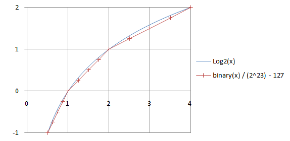
Many computers follow the IEEE (or sufficiently similar) representation, and a very rapid approximation to the square root can be obtained for starting Newton's method. The technique that follows is based on the fact that the floating point format (in base two) approximates the base-2 logarithm. That is $\log _{2}(m\times 2^{p})=p+\log _{2}(m)$

So for a 32-bit single precision floating point number in IEEE format (where notably, the power has a bias of 127 added for the represented form) you can get the approximate logarithm by interpreting its binary representation as a 32-bit integer, scaling it by $2^{-23}$ , and removing a bias of 127, i.e.

x_{\text{int}}\cdot 2^{-23}-127\approx \log _{2}(x).

For example, 1.0 is represented by a hexadecimal number 0x3F800000, which would represent $1065353216=127\cdot 2^{23}$ if taken as an integer. Using the formula above you get $1065353216\cdot 2^{-23}-127=0$ , as expected from $\log _{2}(1.0)$ . In a similar fashion you get 0.5 from 1.5 (0x3FC00000).

To get the square root, divide the logarithm by 2 and convert the value back. The following program demonstrates the idea. Note that the exponent's lowest bit is intentionally allowed to propagate into the mantissa. One way to justify the steps in this program is to assume $b$ is the exponent bias and $n$ is the number of explicitly stored bits in the mantissa and then show that

(((x_{\text{int}}/2^{n}-b)/2)+b)\cdot 2^{n}=(x_{\text{int}}-2^{n})/2+((b+1)/2)\cdot 2^{n}.

/* Assumes that float is in the IEEE 754 single precision floating point format
 * and that int is 32 bits. */
float sqrt_approx(float z)
{
    int val_int = *(int*)&z; /* Same bits, but as an int */
    /*
     * To justify the following code, prove that
     *
     * ((((val_int / 2^m) - b) / 2) + b) * 2^m = ((val_int - 2^m) / 2) + ((b + 1) / 2) * 2^m)
     *
     * where
     *
     * b = exponent bias
     * m = number of mantissa bits
     *
     * .
     */

    val_int -= 1 << 23; /* Subtract 2^m. */
    val_int >>= 1; /* Divide by 2. */
    val_int += 1 << 29; /* Add ((b + 1) / 2) * 2^m. */

    return *(float*)&val_int; /* Interpret again as float */
}

The three mathematical operations forming the core of the above function can be expressed in a single line. An additional adjustment can be added to reduce the maximum relative error. So, the three operations, not including the cast, can be rewritten as

val_int = (1 << 29) + (val_int >> 1) - (1 << 22) + a;

where a is a bias for adjusting the approximation errors. For example, with a = 0 the results are accurate for even powers of 2 (e.g., 1.0), but for other numbers the results will be slightly too big (e.g.,1.5 for 2.0 instead of 1.414... with 6% error). With a = -0x4C000, the errors are between about -3.5% and 3.5%.

If the approximation is to be used for an initial guess for Newton's method to the equation $(1/x^{2})-S=0$ , then the reciprocal form shown in the following section is preferred.

Reciprocal of the square root

Main article: Fast inverse square root

A variant of the above routine is included below, which can be used to compute the reciprocal of the square root, i.e., $x^{-{1 \over 2}}$ instead, was written by Greg Walsh. The integer-shift approximation produced a relative error of less than 4%, and the error dropped further to 0.15% with one iteration of Newton's method on the following line.^[13] In computer graphics it is a very efficient way to normalize a vector.

float invSqrt(float x)
{
    float xhalf = 0.5f*x;
    union
    {
        float x;
        int i;
    } u;
    u.x = x;
    u.i = 0x5f3759df - (u.i >> 1);
    /* The next line can be repeated any number of times to increase accuracy */
    u.x = u.x * (1.5f - xhalf * u.x * u.x);
    return u.x;
}

Some VLSI hardware implements inverse square root using a second degree polynomial estimation followed by a Goldschmidt iteration.^[14]

Negative or complex square

If S < 0, then its principal square root is

{\sqrt {S}}={\sqrt {\vert S\vert }}\,\,i\,.

If S = a+bi where a and b are real and b ≠ 0, then its principal square root is

{\sqrt {S}}={\sqrt {\frac {\vert S\vert +a}{2}}}\,+\,\operatorname {sgn}(b){\sqrt {\frac {\vert S\vert -a}{2}}}\,\,i\,.

This can be verified by squaring the root.^[15]^[16] Here

\vert S\vert ={\sqrt {a^{2}+b^{2}}}

is the modulus of S. The principal square root of a complex number is defined to be the root with the non-negative real part.

Notes

↑ There is no direct evidence showing how the Babylonians computed square roots, although there are informed conjectures. (Square root of 2#Notes gives a summary and references.)
↑ Heath, Thomas (1921). A History of Greek Mathematics, Vol. 2. Oxford: Clarendon Press. pp. 323–324.
↑ Fast integer square root by Mr. Woo's abacus algorithm (archived)
↑ Integer Square Root function
↑ Sri Bharati Krisna Tirthaji (2008) [1965]. Vedic Mathematics or Sixteen Simple Mathematical Formulae from the Vedas. Motilal Banarsidass. ISBN 978-8120801639.
↑ M. V. Wilkes, D. J. Wheeler and S. Gill, "The Preparation of Programs for an Electronic Digital Computer", Addison-Wesley, 1951.
↑ M. Campbell-Kelly, "Origin of Computing", Scientific American, September 2009.
↑ J. C. Gower, "A Note on an Iterative Method for Root Extraction", The Computer Journal 1(3):142–143, 1958.
↑ Peter Markstein (November 2004). "Software Division and Square Root Using Goldschmidt's Algorithms". CiteSeerX 10.1.1.85.9648. Missing or empty |url= (help)
↑ Meher, Pramod Kumar; Valls, Javier; Juang, Tso-Bing; Sridharan, K.; Maharatna, Koushik (2008-08-22). "50 Years of CORDIC: Algorithms, Architectures and Applications" (PDF). IEEE Transactions on Circuits & Systems-I: Regular Papers (published 2009-09-09). 56 (9): 1893–1907. Retrieved 2016-01-03.
↑ Beceanu, Marius. "Period of the Continued Fraction of sqrt(n)" (PDF). Theorem 2.3. Archived from the original (PDF) on 21 December 2015. Retrieved 21 December 2015.
↑ Gliga, Alexandra Ioana (March 17, 2006). On continued fractions of the square root of prime numbers (pdf). Corollary 3.3.
↑ Fast Inverse Square Root by Chris Lomont
↑ "High-Speed Double-Precision Computation of Reciprocal, Division, Square Root and Inverse Square Root" by José-Alejandro Piñeiro and Javier Díaz Bruguera 2002 (abstract)
↑ Abramowitz, Miltonn; Stegun, Irene A. (1964). Handbook of mathematical functions with formulas, graphs, and mathematical tables. Courier Dover Publications. p. 17. ISBN 0-486-61272-4. , Section 3.7.26, p. 17
↑ Cooke, Roger (2008). Classical algebra: its nature, origins, and uses. John Wiley and Sons. p. 59. ISBN 0-470-25952-3. , Extract: page 59

External links

Weisstein, Eric W. "Square root algorithms". MathWorld.

This article is issued from Wikipedia - version of the 11/27/2016. The text is available under the Creative Commons Attribution/Share Alike but additional terms may apply for the media files.

Methods of computing square roots

Rough estimation

Babylonian method

Example

Convergence

Worst case for convergence

Digit-by-digit calculation

Basic principle

Decimal (base 10)

Examples

Binary numeral system (base 2)

Example

Exponential identity

Bakhshali approximation

Example

Vedic duplex method for extracting a square root

Basic principle

Example

A two-variable iterative method

Iterative methods for reciprocal square roots

Goldschmidt’s algorithm

Taylor series

Other methods

Continued fraction expansion

Algorithm

Example, square root of 114 as a continued fraction

Generalized continued fraction

Using Pell's equation

Approximations that depend on the floating point representation

Reciprocal of the square root

Negative or complex square

See also

Notes

External links