Line graph

This article is about the mathematical concept. For the statistical presentation method, see line chart.

Not to be confused with linear graph.

In the mathematical discipline of graph theory, the line graph of an undirected graph G is another graph L(G) that represents the adjacencies between edges of G. The name line graph comes from a paper by Harary & Norman (1960) although both Whitney (1932) and Krausz (1943) used the construction before this.^[1] Other terms used for the line graph include the covering graph, the derivative, the edge-to-vertex dual, the conjugate, the representative graph, and the ϑ-obrazom,^[1] as well as the edge graph, the interchange graph, the adjoint graph, and the derived graph.^[2]

Hassler Whitney (1932) proved that with one exceptional case the structure of a connected graph G can be recovered completely from its line graph.^[3] Many other properties of line graphs follow by translating the properties of the underlying graph from vertices into edges, and by Whitney's theorem the same translation can also be done in the other direction. Line graphs are claw-free, and the line graphs of bipartite graphs are perfect. Line graphs can be characterized by nine forbidden subgraphs, and can be recognized in linear time.

Various generalizations of line graphs have also been studied, including the line graphs of line graphs, line graphs of multigraphs, line graphs of hypergraphs, and line graphs of weighted graphs.

Formal definition

Given a graph G, its line graph L(G) is a graph such that

each vertex of L(G) represents an edge of G; and
two vertices of L(G) are adjacent if and only if their corresponding edges share a common endpoint ("are incident") in G.

That is, it is the intersection graph of the edges of G, representing each edge by the set of its two endpoints.^[2]

Example

The following figures show a graph (left, with blue vertices) and its line graph (right, with green vertices). Each vertex of the line graph is shown labeled with the pair of endpoints of the corresponding edge in the original graph. For instance, the green vertex on the right labeled 1,3 corresponds to the edge on the left between the blue vertices 1 and 3. Green vertex 1,3 is adjacent to three other green vertices: 1,4 and 1,2 (corresponding to edges sharing the endpoint 1 in the blue graph) and 4,3 (corresponding to an edge sharing the endpoint 3 in the blue graph).

Graph G
Vertices in L(G) constructed from edges in G
Added edges in L(G)
The line graph L(G)

Properties

Translated properties of the underlying graph

Properties of a graph G that depend only on adjacency between edges may be translated into equivalent properties in L(G) that depend on adjacency between vertices. For instance, a matching in G is a set of edges no two of which are adjacent, and corresponds to a set of vertices in L(G) no two of which are adjacent, that is, an independent set.^[4]

Thus,

The line graph of a connected graph is connected. If G is connected, it contains a path connecting any two of its edges, which translates into a path in L(G) containing any two of the vertices of L(G). However, a graph G that has some isolated vertices, and is therefore disconnected, may nevertheless have a connected line graph.^[5]
A line graph has an articulation point if and only if the underlying graph has a bridge for which neither endpoint has degree one.^[2]
For a graph G with n vertices and m edges, the number of vertices of the line graph L(G) is m, and the number of edges of L(G) is half the sum of the squares of the degrees of the vertices in G, minus m.^[6]
A maximum independent set in a line graph corresponds to maximum matching in the original graph. Since maximum matchings may be found in polynomial time, so may the maximum independent sets of line graphs, despite the hardness of the maximum independent set problem for more general families of graphs.^[4]
The edge chromatic number of a graph G is equal to the vertex chromatic number of its line graph L(G).^[7]
The line graph of an edge-transitive graph is vertex-transitive. This property can be used to generate families of graphs that (like the Petersen graph) are vertex-transitive but are not Cayley graphs: if G is an edge-transitive graph that has at least five vertices, is not bipartite, and has odd vertex degrees, then L(G) is a vertex-transitive non-Cayley graph.^[8]
If a graph G has an Euler cycle, that is, if G is connected and has an even number of edges at each vertex, then the line graph of G is Hamiltonian. However, not all Hamiltonian cycles in line graphs come from Euler cycles in this way; for instance, the line graph of a Hamiltonian graph G is itself Hamiltonian, regardless of whether G is also Eulerian.^[9]
If two simple graphs are isomorphic then their line graphs are also isomorphic. The Whitney graph isomorphism theorem provides a converse to this for every but one graph.
In the context of complex network theory, the line graph of a random network preserves many of the properties of the network such as the small-world property (the existence of short paths between all pairs of vertices) and the shape of its degree distribution.^[10] Evans & Lambiotte (2009) observe that any method for finding vertex clusters in a complex network can be applied to the line graph and used to cluster its edges instead.

Whitney isomorphism theorem

The diamond graph, an exception to the strong Whitney theorem

If the line graphs of two connected graphs are isomorphic, then the underlying graphs are isomorphic, except in the case of the triangle graph K₃ and the claw K_1,3, which have isomorphic line graphs but are not themselves isomorphic.^[3]

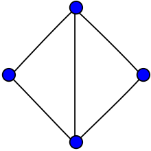
As well as K₃ and K_1,3, there are some other exceptional small graphs with the property that their line graph has a higher degree of symmetry than the graph itself. For instance, the diamond graph K_1,1,2 (two triangles sharing an edge) has four graph automorphisms but its line graph K_1,2,2 has eight. In the illustration of the diamond graph shown, rotating the graph by 90 degrees is not a symmetry of the graph, but is a symmetry of its line graph. However, all such exceptional cases have at most four vertices. A strengthened version of the Whitney isomorphism theorem states that, for connected graphs with more than four vertices, there is a one-to-one correspondence between isomorphisms of the graphs and isomorphisms of their line graphs.^[11]

Analogues of the Whitney isomorphism theorem have been proven for the line graphs of multigraphs, but are more complicated in this case.^[12]

Strongly regular and perfect line graphs

A line perfect graph. The edges in each biconnected component are colored black if the component is bipartite, blue if the component is a tetrahedron, and red if the component is a book of triangles.

The line graph of the complete graph K_n is also known as the triangular graph, the Johnson graph J(n,2), or the complement of the Kneser graph KG_n,2. Triangular graphs are characterized by their spectra, except for n = 8.^[13] They may also be characterized (again with the exception of K₈) as the strongly regular graphs with parameters srg(n(n − 1)/2, 2(n − 2), n − 2, 4).^[14] The three strongly regular graphs with the same parameters and spectrum as L(K₈) are the Chang graphs, which may be obtained by graph switching from L(K₈).

The line graph of a bipartite graph is perfect (see König's theorem). The line graphs of bipartite graphs form one of the key building blocks of perfect graphs, used in the proof of the strong perfect graph theorem.^[15] A special case of these graphs are the rook's graphs, line graphs of complete bipartite graphs. Like the line graphs of complete graphs, they can be characterized with one exception by their numbers of vertices, numbers of edges, and number of shared neighbors for adjacent and non-adjacent points. The one exceptional case is L(K_4,4), which shares its parameters with the Shrikhande graph. When both sides of the bipartition have the same number of vertices, these graphs are again strongly regular.^[16]

More generally, a graph G is said to be line perfect if L(G) is a perfect graph. The line perfect graphs are exactly the graphs that do not contain a simple cycle of odd length greater than three.^[17] Equivalently, a graph is line perfect if and only if each of its biconnected components is either bipartite or of the form K₄ (the tetrahedron) or K_1,1,n (a book of one or more triangles all sharing a common edge).^[18] Every line perfect graph is itself perfect.^[19]

Other related graph families

All line graphs are claw-free graphs, graphs without an induced subgraph in the form of a three-leaf tree.^[20] As with claw-free graphs more generally, every connected line graph L(G) with an even number of edges has a perfect matching;^[21] equivalently, this means that if the underlying graph G has an even number of edges, its edges can be partitioned into two-edge paths.

The line graphs of trees are exactly the claw-free block graphs.^[22] These graphs have been used to solve a problem in extremal graph theory, of constructing a graph with a given number of edges and vertices whose largest tree induced as a subgraph is as small as possible.^[23]

All eigenvalues of the adjacency matrix of a line graph are at least −2.For this reason, the graphs whose eigenvalues have this property have been called generalized line graphs.^[24]

Characterization and recognition

Clique partition

Partition of a line graph into cliques

For an arbitrary graph G, and an arbitrary vertex v in G, the set of edges incident to v corresponds to a clique in the line graph L(G). The cliques formed in this way partition the edges of L(G). Each vertex of L(G) belongs to exactly two of them (the two cliques corresponding to the two endpoints of the corresponding edge in G).

The existence of such a partition into cliques can be used to characterize the line graphs: A graph L is the line graph of some other graph or multigraph if and only if it is possible to find a collection of cliques in L (allowing some of the cliques to be single vertices) that partition the edges of L, such that each vertex of L belongs to exactly two of the cliques.^[20] It is the line graph of a graph (rather than a multigraph) if this set of cliques satisfies the additional condition that no two vertices of L are both in the same two cliques. Given such a family of cliques, the underlying graph G for which L is the line graph can be recovered by making one vertex in G for each clique, and an edge in G for each vertex in L with its endpoints being the two cliques containing the vertex in L. By the strong version of Whitney's isomorphism theorem, if the underlying graph G has more than four vertices, there can be only one partition of this type.

For example, this characterization can be used to show that the following graph is not a line graph:

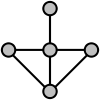
In this example, the edges going upward, to the left, and to the right from the central degree-four vertex do not have any cliques in common. Therefore, any partition of the graph's edges into cliques would have to have at least one clique for each of these three edges, and these three cliques would all intersect in that central vertex, violating the requirement that each vertex appear in exactly two cliques. Thus, the graph shown is not a line graph.

Forbidden subgraphs

The nine minimal non-line graphs, from Beineke's forbidden-subgraph characterization of line graphs. A graph is a line graph if and only if it does not contain one of these nine graphs as an induced subgraph.

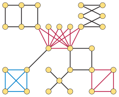
An alternative characterization of line graphs was proven by Beineke (1970) (and reported earlier without proof by Beineke (1968)). He showed that there are nine minimal graphs that are not line graphs, such that any graph that is not a line graph has one of these nine graphs as an induced subgraph. That is, a graph is a line graph if and only if no subset of its vertices induces one of these nine graphs. In the example above, the four topmost vertices induce a claw (that is, a complete bipartite graph K_1,3), shown on the top left of the illustration of forbidden subgraphs. Therefore, by Beineke's characterization, this example cannot be a line graph. For graphs with minimum degree at least 5, only the six subgraphs in the left and right columns of the figure are needed in the characterization.^[25] Line graphs of multigraphs may be similarly characterized by three of Beineke's nine forbidden subgraphs.^[26]

Algorithms

Roussopoulos (1973) and Lehot (1974) described linear time algorithms for recognizing line graphs and reconstructing their original graphs. Sysło (1982) generalized these methods to directed graphs. Degiorgi & Simon (1995) described an efficient data structure for maintaining a dynamic graph, subject to vertex insertions and deletions, and maintaining a representation of the input as a line graph (when it exists) in time proportional to the number of changed edges at each step.

The algorithms of Roussopoulos (1973) and Lehot (1974) are based on characterizations of line graphs involving odd triangles (triangles in the line graph with the property that there exists another vertex adjacent to an odd number of triangle vertices). However, the algorithm of Degiorgi & Simon (1995) uses only Whitney's isomorphism theorem. It is complicated by the need to recognize deletions that cause the remaining graph to become a line graph, but when specialized to the static recognition problem only insertions need to be performed, and the algorithm performs the following steps:

Construct the input graph L by adding vertices one at a time, at each step choosing a vertex to add that is adjacent to at least one previously-added vertex. While adding vertices to L, maintain a graph G for which L = L(G); if the algorithm ever fails to find an appropriate graph G, then the input is not a line graph and the algorithm terminates.
When adding a vertex v to a graph L(G) for which G has four or fewer vertices, it might be the case that the line graph representation is not unique. But in this case, the augmented graph is small enough that a representation of it as a line graph can be found by a brute force search in constant time.
When adding a vertex v to a larger graph L that equals the line graph of another graph G, let S be the subgraph of G formed by the edges that correspond to the neighbors of v in L. Check that S has a vertex cover consisting of one vertex or two non-adjacent vertices. If there are two vertices in the cover, augment G by adding an edge (corresponding to v) that connects these two vertices. If there is only one vertex in the cover, then add a new vertex to G, adjacent to this vertex.

Each step either takes constant time, or involves finding a vertex cover of constant size within a graph S whose size is proportional to the number of neighbors of v. Thus, the total time for the whole algorithm is proportional to the sum of the numbers of neighbors of all vertices, which (by the handshaking lemma) is proportional to the number of input edges.

Iterating the line graph operator

van Rooij & Wilf (1965) consider the sequence of graphs

G,L(G),L(L(G)),L(L(L(G))),\dots .\

They show that, when G is a finite connected graph, only four behaviors are possible for this sequence:

If G is a cycle graph then L(G) and each subsequent graph in this sequence is isomorphic to G itself. These are the only connected graphs for which L(G) is isomorphic to G.^[27]
If G is a claw K_1,3, then L(G) and all subsequent graphs in the sequence are triangles.
If G is a path graph then each subsequent graph in the sequence is a shorter path until eventually the sequence terminates with an empty graph.
In all remaining cases, the sizes of the graphs in this sequence eventually increase without bound.

If G is not connected, this classification applies separately to each component of G.

For connected graphs that are not paths, all sufficiently high numbers of iteration of the line graph operation produce graphs that are Hamiltonian.^[28]

Generalizations

Medial graphs and convex polyhedra

Main article: Medial graph

When a planar graph G has maximum vertex degree three, its line graph is planar, and every planar embedding of G can be extended to an embedding of L(G). However, there exist planar graphs with higher degree whose line graphs are nonplanar. These include, for example, the 5-star K_1,5, the gem graph formed by adding two non-crossing diagonals within a regular pentagon, and all convex polyhedra with a vertex of degree four or more.^[29]

An alternative construction, the medial graph, coincides with the line graph for planar graphs with maximum degree three, but is always planar. It has the same vertices as the line graph, but potentially fewer edges: two vertices of the medial graph are adjacent if and only if the corresponding two edges are consecutive on some face of the planar embedding. The medial graph of the dual graph of a plane graph is the same as the medial graph of the original plane graph.^[30]

For regular polyhedra or simple polyhedra, the medial graph operation can be represented geometrically by the operation of cutting off each vertex of the polyhedron by a plane through the midpoints of all its incident edges.^[31] This operation is known variously as the second truncation,^[32] degenerate truncation,^[33] or rectification.^[34]

Total graphs

The total graph T(G) of a graph G has as its vertices the elements (vertices or edges) of G, and has an edge between two elements whenever they are either incident or adjacent. The total graph may also be obtained by subdividing each edge of G and then taking the square of the subdivided graph.^[35]

Multigraphs

The concept of the line graph of G may naturally be extended to the case where G is a multigraph. In this case, the characterizations of these graphs can be simplified: the characterization in terms of clique partitions no longer needs to prevent two vertices from belonging to the same to cliques, and the characterization by forbidden graphs has fewer forbidden graphs.^[26]

However, for multigraphs, there are larger numbers of pairs of non-isomorphic graphs that have the same line graphs. For instance a complete bipartite graph K_1,n has the same line graph as the dipole graph and Shannon multigraph with the same number of edges. Nevertheless, analogues to Whitney's isomorphism theorem can still be derived in this case.^[12]

Line digraphs

Construction of the de Bruijn graphs as iterated line digraphs

It is also possible to generalize line graphs to directed graphs.^[36] If G is a directed graph, its directed line graph or line digraph has one vertex for each edge of G. Two vertices representing directed edges from u to v and from w to x in G are connected by an edge from uv to wx in the line digraph when v = w. That is, each edge in the line digraph of G represents a length-two directed path in G. The de Bruijn graphs may be formed by repeating this process of forming directed line graphs, starting from a complete directed graph.^[37]

Weighted line graphs

In a line graph L(G), each vertex of degree k in the original graph G creates k(k-1)/2 edges in the line graph. For many types of analysis this means high degree nodes in G are over represented in the line graph L(G). For instance consider a random walk on the vertices of the original graph G. This will pass along some edge e with some frequency f. On the other hand, this edge e is mapped to a unique vertex, say v, in the line graph L(G). If we now perform the same type of random walk on the vertices of the line graph, the frequency with which v is visited can be completely different from f. If our edge e in G was connected to nodes of degree O(k), it will be traversed O(k²) more frequently in the line graph L(G). Put another way, the Whitney graph isomorphism theorem guarantees that the line graph almost always encodes the topology of the original graph G faithfully but it does not guarantee that dynamics on these two graphs have a simple relationship. One solution is to construct a weighted line graph, that is, a line graph with weighted edges. There are several natural ways to do this.^[38] For instance if edges d and e in the graph G are incident at a vertex v with degree k, then in the line graph L(G) the edge connecting the two vertices d and e can be given weight 1/(k-1). In this way every edge in G (provided neither end is connected to a vertex of degree '1') will have strength 2 in the line graph L(G) corresponding to the two ends that the edge has in G. It is straightforward to extend this definition of a weighted line graph to cases where the original graph G was directed or even weighted.^[39] The principle in all cases is to ensure the line graph L(G) reflects the dynamics as well as the topology of the original graph G.

Line graphs of hypergraphs

Main article: Line graph of a hypergraph

The edges of a hypergraph may form an arbitrary family of sets, so the line graph of a hypergraph is the same as the intersection graph of the sets from the family.^[25]

Notes

1 2 Hemminger & Beineke (1978), p. 273.
1 2 3 Harary (1972), p. 71.
1 2 Whitney (1932); Krausz (1943); Harary (1972), Theorem 8.3, p. 72. Harary gives a simplified proof of this theorem by Jung (1966).
1 2 Paschos, Vangelis Th. (2010), Combinatorial Optimization and Theoretical Computer Science: Interfaces and Perspectives, John Wiley & Sons, p. 394, ISBN 9780470393673, Clearly, there is a one-to-one correspondence between the matchings of a graph and the independent sets of its line graph.
↑ The need to consider isolated vertices when considering the connectivity of line graphs is pointed out by Cvetković, Rowlinson & Simić (2004), p. 32.
↑ Harary (1972), Theorem 8.1, p. 72.
↑ Diestel, Reinhard (2006), Graph Theory, Graduate Texts in Mathematics, 173, Springer, p. 112, ISBN 9783540261834 . Also in free online edition, Chapter 5 ("Colouring"), p. 118.
↑ Lauri, Josef; Scapellato, Raffaele (2003), Topics in graph automorphisms and reconstruction, London Mathematical Society Student Texts, 54, Cambridge: Cambridge University Press, p. 44, ISBN 0-521-82151-7, MR 1971819 . Lauri and Scapellato credit this result to Mark Watkins.
↑ Harary (1972), Theorem 8.8, p. 80.
↑ Ramezanpour, Karimipour & Mashaghi (2003).
↑ Jung (1966); Degiorgi & Simon (1995).
1 2 Zverovich (1997)
↑ van Dam, Edwin R.; Haemers, Willem H. (2003), "Which graphs are determined by their spectrum?", Linear Algebra and its Applications, 373: 241–272, doi:10.1016/S0024-3795(03)00483-X, MR 2022290 . See in particular Proposition 8, p. 262.
↑ Harary (1972), Theorem 8.6, p. 79. Harary credits this result to independent papers by L. C. Chang (1959) and A. J. Hoffman (1960).
↑ Chudnovsky, Maria; Robertson, Neil; Seymour, Paul; Thomas, Robin (2006), "The strong perfect graph theorem", Annals of Mathematics, 164 (1): 51–229, doi:10.4007/annals.2006.164.51 . See also Roussel, F.; Rusu, I.; Thuillier, H. (2009), "The strong perfect graph conjecture: 40 years of attempts, and its resolution", Discrete Mathematics, 309 (20): 6092–6113, doi:10.1016/j.disc.2009.05.024, MR 2552645 .
↑ Harary (1972), Theorem 8.7, p. 79. Harary credits this characterization of line graphs of complete bipartite graphs to Moon and Hoffman. The case of equal numbers of vertices on both sides had previously been proven by Shrikhande.
↑ Trotter (1977); de Werra (1978).
↑ Maffray (1992).
↑ Trotter (1977).
1 2 Harary (1972), Theorem 8.4, p. 74, gives three equivalent characterizations of line graphs: the partition of the edges into cliques, the property of being claw-free and odd diamond-free, and the nine forbidden graphs of Beineke.
↑ Sumner, David P. (1974), "Graphs with 1-factors", Proceedings of the American Mathematical Society, American Mathematical Society, 42 (1): 8–12, doi:10.2307/2039666, JSTOR 2039666, MR 0323648 . Las Vergnas, M. (1975), "A note on matchings in graphs", Cahiers du Centre d'Études de Recherche Opérationnelle, 17 (2-3-4): 257–260, MR 0412042 .
↑ Harary (1972), Theorem 8.5, p. 78. Harary credits the result to Gary Chartrand.
↑ Erdős, Paul; Saks, Michael; Sós, Vera T. (1986), "Maximum induced trees in graphs", Journal of Combinatorial Theory, Series B, 41 (1): 61–79, doi:10.1016/0095-8956(86)90028-6 .
↑ Cvetković, Rowlinson & Simić (2004).
1 2 Metelsky & Tyshkevich (1997)
1 2 Harary (1972), Exercise 8.14, p. 83.
↑ This result is also Theorem 8.2 of Harary (1972).
↑ Harary (1972), Theorem 8.11, p. 81. Harary credits this result to Gary Chartrand.
↑ Sedláček (1964); Greenwell & Hemminger (1972).
↑ Archdeacon, Dan (1992), "The medial graph and voltage-current duality", Discrete Mathematics, 104 (2): 111–141, doi:10.1016/0012-365X(92)90328-D, MR 1172842 .
↑ McKee, T. A. (1989), "Graph-theoretic model of geographic duality", Combinatorial Mathematics: Proceedings of the Third International Conference (New York, 1985), Ann. New York Acad. Sci., 555, New York: New York Acad. Sci., pp. 310–315, doi:10.1111/j.1749-6632.1989.tb22465.x, MR 1018637 .
↑ Pugh, Anthony (1976), Polyhedra: A Visual Approach, University of California Press, ISBN 9780520030565 .
↑ Loeb, Arthur Lee (1991), Space Structures—their Harmony and Counterpoint (5th ed.), Birkhäuser, ISBN 9783764335885 .
↑ Weisstein, Eric W. "Rectification". MathWorld.
↑ Harary (1972), p. 82.
↑ Harary & Norman (1960).
↑ Zhang & Lin (1987).
↑ Evans & Lambiotte (2009).
↑ Evans & Lambiotte (2010).

References

Beineke, L. W. (1968), "Derived graphs of digraphs", in Sachs, H.; Voss, H.-J.; Walter, H.-J., Beiträge zur Graphentheorie, Leipzig: Teubner, pp. 17–33 .
Beineke, L. W. (1970), "Characterizations of derived graphs", Journal of Combinatorial Theory, 9 (2): 129–135, doi:10.1016/S0021-9800(70)80019-9, MR 0262097 .
Cvetković, Dragoš; Rowlinson, Peter; Simić, Slobodan (2004), Spectral generalizations of line graphs, London Mathematical Society Lecture Note Series, 314, Cambridge: Cambridge University Press, doi:10.1017/CBO9780511751752, ISBN 0-521-83663-8, MR 2120511 .
Degiorgi, Daniele Giorgio; Simon, Klaus (1995), "A dynamic algorithm for line graph recognition", Graph-theoretic concepts in computer science (Aachen, 1995), Lecture Notes in Computer Science, 1017, Berlin: Springer, pp. 37–48, doi:10.1007/3-540-60618-1_64, MR 1400011 .
Evans, T.S.; Lambiotte, R. (2009), "Line graphs, link partitions and overlapping communities", Physical Review E, 80: 016105, arXiv:0903.2181, doi:10.1103/PhysRevE.80.016105 .
Evans, T.S.; Lambiotte, R. (2010), "Line Graphs of Weighted Networks for Overlapping Communities", European Physical Journal B, 77: 265–272, arXiv:0912.4389, doi:10.1140/epjb/e2010-00261-8 .
Greenwell, D. L.; Hemminger, Robert L. (1972), "Forbidden subgraphs for graphs with planar line graphs", Discrete Mathematics, 2: 31–34, doi:10.1016/0012-365X(72)90058-1, MR 0297604 .
Harary, F.; Norman, R. Z. (1960), "Some properties of line digraphs", Rendiconti del Circolo Matematico di Palermo, 9 (2): 161–169, doi:10.1007/BF02854581 .
Harary, F. (1972), "8. Line Graphs", Graph Theory (PDF), Massachusetts: Addison-Wesley, pp. 71–83 .
Hemminger, R. L.; Beineke, L. W. (1978), "Line graphs and line digraphs", in Beineke, L. W.; Wilson, R. J., Selected Topics in Graph Theory, Academic Press Inc., pp. 271–305 .
Jung, H. A. (1966), "Zu einem Isomorphiesatz von H. Whitney für Graphen", Mathematische Annalen (in German), 164: 270–271, doi:10.1007/BF01360250, MR 0197353 .
Krausz, J. (1943), "Démonstration nouvelle d'un théorème de Whitney sur les réseaux", Mat. Fiz. Lapok, 50: 75–85, MR 0018403 .
Lehot, Philippe G. H. (1974), "An optimal algorithm to detect a line graph and output its root graph", Journal of the ACM, 21: 569–575, doi:10.1145/321850.321853, MR 0347690 .
Maffray, Frédéric (1992), "Kernels in perfect line-graphs", Journal of Combinatorial Theory, Series B, 55 (1): 1–8, doi:10.1016/0095-8956(92)90028-V, MR 1159851 .
Metelsky, Yury; Tyshkevich, Regina (1997), "On line graphs of linear 3-uniform hypergraphs", Journal of Graph Theory, 25 (4): 243–251, doi:10.1002/(SICI)1097-0118(199708)25:4<243::AID-JGT1>3.0.CO;2-K .
Ramezanpour, A.; Karimipour, V.; Mashaghi, A. (2003), "Generating correlated networks from uncorrelated ones", Phys. Rev. E, 67: 046107, doi:10.1103/physreve.67.046107 .
van Rooij, A. C. M.; Wilf, H. S. (1965), "The interchange graph of a finite graph", Acta Mathematica Hungarica, 16 (3–4): 263–269, doi:10.1007/BF01904834 .
Roussopoulos, N. D. (1973), "A max {m,n} algorithm for determining the graph H from its line graph G", Information Processing Letters, 2 (4): 108–112, doi:10.1016/0020-0190(73)90029-X, MR 0424435 .
Sedláček, J. (1964), "Some properties of interchange graphs", Theory of Graphs and its Applications (Proc. Sympos. Smolenice, 1963), Publ. House Czechoslovak Acad. Sci., Prague, pp. 145–150, MR 0173255 .
Sysło, Maciej M. (1982), "A labeling algorithm to recognize a line digraph and output its root graph", Information Processing Letters, 15 (1): 28–30, doi:10.1016/0020-0190(82)90080-1, MR 678028 .
Trotter, L. E., Jr. (1977), "Line perfect graphs", Mathematical Programming, 12 (2): 255–259, doi:10.1007/BF01593791, MR 0457293 .
de Werra, D. (1978), "On line perfect graphs", Mathematical Programming, 15 (2): 236–238, doi:10.1007/BF01609025, MR 509968 .
Whitney, H. (1932), "Congruent graphs and the connectivity of graphs", American Journal of Mathematics, 54 (1): 150–168, doi:10.2307/2371086, JSTOR 2371086 .
Zhang, Fu Ji; Lin, Guo Ning (1987), "On the de Bruijn–Good graphs", Acta Math. Sinica, 30 (2): 195–205, MR 0891925 .
Зверович, И. Э. (1997), Аналог теоремы Уитни для реберных графов мультиграфов и реберные мультиграфы, Diskretnaya Matematika (in Russian), 9 (2): 98–105, doi:10.4213/dm478, MR 1468075 . Translated into English as Zverovich, I. È. (1997), "An analogue of the Whitney theorem for edge graphs of multigraphs, and edge multigraphs", Discrete Mathematics and Applications, 7 (3): 287–294, doi:10.1515/dma.1997.7.3.287 .

External links

line graphs, Information System on Graph Class Inclusions External link in |publisher= (help) (last visited Sep 23 2013)
Weisstein, Eric W. "Line Graph". MathWorld.

This article is issued from Wikipedia - version of the 10/19/2016. The text is available under the Creative Commons Attribution/Share Alike but additional terms may apply for the media files.