Kolmogorov–Zurbenko filter

The Kolmogorov–Zurbenko (KZ) filter was first proposed by A. N. Kolmogorov and formally defined by Zurbenko.^[1] It is a series of iterations of a moving average filter of length m, where m is a positive, odd integer. The KZ filter belongs to the class of low-pass filters. The KZ filter has two parameters, the length m of the moving average window and the number of iterations k of the moving average itself. It also can be considered as a special window function designed to eliminate spectral leakage.

Andrey Kolmogorov and Igor Zurbenko on a research ship in the Pacific.

Andrey Kolmogorov and Igor Zurbenko

Background

A. N. Kolmogorov had the original idea for the KZ filter during a study of turbulence in the Pacific Ocean.^[1] Kolmogorov had just received the International Balzan Prize for his law of 5/3 in the energy spectra of turbulence. Surprisingly the 5/3 law was not obeyed in the Pacific Ocean, causing great concern. Standard Fast Fourier Transform (FFT) was completely fooled by the noisy and non-stationary ocean environment. KZ filtration resolved the problem and enabled proof of Kolmogorov's law in that domain. Filter construction relied on the main concepts of the continuous Fourier transform and their discrete analogues. The algorithm of the KZ filter came from the definition of higher-order derivatives for discrete functions as higher-order differences. Believing that infinite smoothness in the Gaussian window was a beautiful but unrealistic approximation of a truly discrete world, Kolmogorov chose a finitely differentiable tapering window with finite support, and created this mathematical construction for the discrete case.^[1] The KZ filter is robust and nearly optimal. Because its operation is a simple Moving Average (MA), the KZ filter performs well in a missing data environment, especially in multidimensional time series where missing data problem arises from spatial sparseness. Another nice feature of the KZ filter is that the two parameters have clear interpretation so that it can be easily adopted by specialists in different areas. A few software packages for time series, longitudinal and spatial data have been developed in the popular statistical software R, which facilitate the use of the KZ filter and its extensions in different areas.

Definition

KZ Filter

Let ${X(t)},t=0,\pm 1,\pm 2,\dots$ be a real-valued time series, the KZ filter with parameters $m$ and $k$ is defined as

KZ_{m,k}[X(t)]=\sum _{s=-k(m-1)/2}^{k(m-1)/2}{X(t+s)\times {a_{s}^{m,k}}}

where coefficients

a_{s}^{{m,k}}={\frac {c_{s}^{{k,m}}}{m^{k}}},s={\frac {-k(m-1)}{2}},\dots ,{\frac {k(m-1)}{2}}

are given by the polynomial coefficients obtained from equation

\sum _{r=0}^{k(m-1)}{z^{r}c_{r-k(m-1)/2}^{k,m}=(1+z+\dots +z^{m-1})^{k}}

From another point of view, the KZ filter with parameters $m$ and $k$ can be defined as $k$ time iterations of a moving average (MA) filter of $m$ points. It can be obtained through iterations.

First iteration is to apply a MA filter over process $X(t)$

KZ_{m,k=1}[X(t)]=\sum _{s=-(m-1)/2}^{(m-1)/2}{X(t+s)}\times {\frac {1}{m}}

The second iteration is to apply the MA operation to the result of the first iteration,

{\begin{aligned}&KZ_{m,k=2}[X(t)]=\sum _{s=-(m-1)/2}^{(m-1)/2}{KZ_{m,k=1}[X(t+s)]\times {\frac {1}{m}}}\\={}&\sum _{s=-2(m-1)/2}^{2(m-1)/2}{X(t+s)\times {a_{s}^{m,k=2}}}\end{aligned}}

Generally the kth iteration is an application of the MA filter to the (k-1)th iteration. The iteration process of a simple operation of MA is very convenient computationally.

Properties

The impulse response function of the product of filters is the convolution of impulse responses. The coefficients of the KZ filter $a m, k s$ , can be interpreted as a distribution obtained by the convolution of k uniform discrete distributions on the interval $[ -(m - 1)/2 , (m - 1)/2 ]$ where m is an odd integer. Therefore, the coefficient $a$ forms a tapering window which has finite support $[ (m - 1)k + 1]$ . The KZ filter $a$ has main weight concentrated on a length of $m \sqrt k$ with weights vanishing to zero outside. The impulse response function of the KZ filter has $k - 2$ continuous derivatives and is asymptotically Gaussian distributed. Zero derivatives at the edges for the impulse response function make from it a sharply declining function, what is resolving in high frequency resolution. The energy transfer function of the KZ filter is

|B_{m,k}(\omega )|^{2}=\left\{{\frac {1}{m}}{\frac {\sin(\pi m\omega )}{\sin(\pi \omega )}}\right\}^{2k}.

It is a low-pass filter with a cut-off frequency of

\omega _{0}\approx {\frac {\sqrt {6}}{\pi }}{\sqrt {\frac {1-(1/2)^{1/2k}}{m^{2}-(1/2)^{1/2k}}}}.

Figure 1.Transfer function of filter for k = 1.

Compared to a MA filter, the KZ filter has much better performance in terms of attenuating the frequency components above the cutoff frequency. The KZ filter is essentially a repetitive MA filter. It is easy to compute and allows for a straightforward way to deal with missing data. The main piece of this procedure is a simple average of available information within the interval of m points disregarding the missing observations within the interval. The same idea can be easily extended to spatial data analysis. It has been shown that missing values have very little effect on the transfer function of the KZ filter.

Arbitrary k will provide k power of this transfer function and will reduce side lobe value to $0.05 k$ . It will be a perfect low pass filter. For practical purposes a choice of k within a range 3 to 5 is usually sufficient, when regular MA (k = 1) is providing strong spectral leakage of about 5%.

Optimality

The KZ filter is robust and nearly optimal. Because its operation is a simple moving average, the KZ filter performs well in a missing data environment, especially in multidimensional time and space where missing data can cause problems arising from spatial sparseness. Another nice feature of the KZ filter is that the two parameters each have clear interpretations so that it can be easily adopted by specialists in different areas. Software implementations for time series, longitudinal and spatial data have been developed in the popular statistical package R, which facilitate the use of the KZ filter and its extensions in different areas.

KZ filter can be used to smooth the periodogram. For a class of stochastic processes, Zurbenko^[1] considered the worst-case scenario where the only information available about a process is its spectral density and smoothness quantified by Hölder condition. He derived the optimal bandwidth of the spectral window, which is dependent upon the underlying smoothness of the spectral density. Zurbenko^[1] compared the performance of Kolmogorov-Zurbenko (KZ) window to the other typically used spectral windows including Bartlett window, Parzen window, Tukey-Hamming window and uniform window and showed that the result from KZ window is closest to optimum.

Developed as an abstract discrete construction, KZ filtration is robust and statistically nearly optimal.^[1] At the same time, because of its natural form, it has computational advantages, permitting analysis of space/time problems with data that has much as 90% of observations missing, and which represent a messy combination of several different physical phenomena.^[2] Clear answers can often be found for "unsolvable" problems.^[2]^[3] Unlike some mathematical developments, KZ is adaptable by specialists in different areas because it has a clear physical interpretation behind it.^[2]^[3]

Extensions

Figure 2: Logarithm of the transfer function for the

KZFT m, k

filter with

ν 0 = .04, m = 100, and k = 1

(black) or

k = 5

(red).

Figure 3: The spectrum of the signal that is the summation of two sine waves about frequencies 0.08 and 0.10 cycles per unit time plus noise N(0,16) with 70% missing values. Adaptively smoothed KZP algorithm was used to determine the spectrum of the simulated data set.

Figure 4: The reconstructed signal that is the sum of two sine waves about frequencies 0.08 and 0.10 cycles per unit time from an original signal with added noise ~N(0, 16) and where 60% of the values were not available.

Extensions of KZ filter include KZ adaptive (KZA) filter,^[1] spatial KZ filter and KZ Fourier transform (KZFT). Yang and Zurbenko^[3] provided a detailed review of KZ filter and its extensions. R packages are also available to implement KZ filtration^[3]^[4]^[5]^[6]

KZFT

KZFT filter is design for a reconstruction of periodic signals or seasonality covered by heavy noise. Seasonality is one of the key forms of nonstationarity that is often seen in time series. It is usually defined as the periodic components within the time series. Spectral analysis is a powerful tool to analyze time series with seasonality. If a process is stationary, its spectrum is a continuous form as well. It can be treated parametrically for simplicity of prediction. If a spectrum contains lines, it indicates that the process is not stationary and contains periodicities. In this situation, parametric fitting generally results in seasonal residuals with reduced energies. This is due to the season to season variations. To avoid this problem, nonparametric approaches including band pass filters are recommended.^[3] Kolmogorov-Zurbenko Fourier Transform (KZFT) is one of such filters. The purpose of many applications is to reconstruct high resolution wavelet from the noisy environment. It was proven that KZFT provides the best possible resolution in spectral domain. It permits the separation of two signals on the edge of a theoretically smallest distance, or reconstruct periodic signals covered by heavy noise and irregularly observed in time.^[3]^[7] Because of this, KZFT provides a unique opportunity for various applications. A computer algorithm to implement the KZFT has been provided in the R software. The KZFT is essentially a band pass filter that belongs to the category of Short-time Fourier transform (STFT) with a unique time window.

KZFT readily uncovers small deviations from a constant spectral density of white noise resulting from computer random numbers generator. Such computer random number generations become predictable in the long run. Kolmogorov complexity provides the opportunity to generate unpredictable sequences of random numbers.^[8]

Formally, we have a process $X (t)$ , $t = ...,-1,0,1,...$ , the KZFT filter with parameters m and k, computed at frequency ν₀, produces an output process, which is defined as following:

KZFT_{m,k,\nu _{0}}[X(t)]=\sum _{s=-k(m-1)/2}^{k(m-1)/2}{X(t+s)\times {a_{s}^{m,k}\times {e^{-i(2m\nu _{0})s}}}}

where $a m, k s$ is defined as: $a m, k s = C m, k s / m k$ , $s = -k(m - 1) / 2$ ,..., $-k(m - 1) / 2$ and the polynomial coefficients $C m, k s$ is given by $Σ k(m-1) r=0 z r C k,m r-k(m-1)/2 = (1 + z + ... + z (m - 1)) k$ . Apparently $KZFT m,k,ν 0 (t) [X (t)]$ filter is equivalent to the application of $KZFT m,k (t)$ filter to the process $X (t + s) e - i 2(mν 0) s$ . Similarly, the KZFT filter can be obtained through iterations in the same way as KZ filter.

The average of the square of KZFT in time over S periods of $ρ 0 = 1 / ν 0$ will provide an estimate of the square amplitude of the wave at frequency ν₀ or KZ periodogram (KZP) based on 2Sρ₀ observations around moment t:

KZP(t,m,k,\nu _{0})=2|{\frac {1}{2S\rho _{0}}}\sum _{\tau =-S\rho _{0}}^{S\rho _{0}}2\operatorname {Re} [KZFT_{m,k,\nu +0}[X(\tau +t)]]^{2}|

Transfer function of KZFT is provided in Figure 2 has a very sharp frequency resolution with bandwidth limited by $c /(m \sqrt k)$ . For a complex-valued process $X (t) = e i(2m ν 0)t$ , the $KZFT m,k, ν 0 (t)$ outcome is unchanged. For a real-valued process, it distributes energy evenly over the real and complex domains. In other words, $2Re[KZFT m,k, ν 0 (t)]$ reconstructs a cosine or sine wave at the same frequency ν₀. It follows that $2Re[KZFT m,k, ν 0 (t)]$ correctly reconstructs the amplitude and phase of an unknown wave with frequency ν₀. Figure below is providing power transfer function of KZFT filtration. It clearly display that it perfectly captured frequency of interest ν₀ = 0.4 and provide practically no spectral leakage from a side lobes which control by parameter k of filtration. For practical purposes choice of k within range 3-5 is usually sufficient, when regular FFT (k=1) is providing strong leakage of about 5%.

Example: Simulated Signal
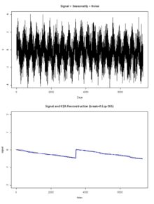
$sin 2 π (0.10) t + sin 2 π (0.02) t +$ normal random noise N(0,16) was used to test the KZFT algorithm’s ability to accurately determine spectra of datasets with missing values. For practical considerations, the percentage of missing values was used at p=70% to determine if the spectrum could continue to capture the dominant frequencies. Using a wider window length of m=600 and k=3 iterations, adaptively smoothed KZP algorithm was used to determine the spectrum for the simulated longitudinal dataset. It is apparent in Figure 3 that the dominant frequencies of 0.08 and 0.10 cycles per unit time are identifiable as the signal’s inherent frequencies.

KZFT reconstruction of original signal embedded in the high noise of longitudinal observations ( missing rate 60%.) The KZFT filter in the KZA package of R-software has a parameter f = frequency. By defining this parameter for each of the known dominant frequencies found in the spectrum, KZFT filter with parameters m=300 and k=3 to reconstruct the signal about each frequency (0.08 and 0.10 cycles per unit time). The reconstructed signal was determined by applying the KZFT filter twice (once about each dominant frequency) and then the summing the results of each filter. The correlation between the true signal and the reconstructed signal was 96.4%; displayed in figure 4. The original observations provide no guess of the complex, hidden periodicity, which was perfectly reconstructed by the algorithm.

Raw data frequently contain hidden frequencies. Combinations of a few fixed frequency waves can complicate the recognition of the mixture of signals, but still remain predictable over time. Publications^[3]^[7] show that atmospheric pressure contains hidden periodicities resulting from the gravitational force of the moon and the daily period of the sun. The reconstruction of these periodic signals of atmospheric tidal waves allows for an explanation and prediction of many anomalies present in extreme weather. Similar tidal waves must exist on the sun resulting from the gravitational force of planets. The rotation of the sun around its axes will cause a current, similar to the equatorial current on the earth. Perturbations or eddies around the current will cause anomalies on the surface of the sun. Horizontal rotational eddies in highly magnetic plasma will create a vertical explosion which will transport deeper, hotter plasma to above the surface of the sun. Each planet creates a tidal wave with a specific frequency on the sun. At times any two of the waves will occur in phase and other times will be out of phase. The resulting amplitude will oscillate with a difference frequency. The estimation of the spectra of sunspot data using the DZ algorithm^[3]^[7] provides two sharp frequency lines with periodicities close to 9.9 and 11.7 years. These frequency lines can be considered as difference frequencies caused by Jupiter and Saturn (9.9) and Venus and Earth (11.7). The difference frequency between 9.9 and 11.7 yields a frequency with a 64-year period. All of these periods are identifiable in sunspot data. The 64-year period component is currently in a declining mode.^[3]^[4] This decline may cause a cooling effect on the earth in the near future. An examination of the joint effect of multiple planets may reveal some long periods in sun activity and help explain climate fluctuations on earth.

KZA

Figure 5a: Plot of signal + seasonality + noise. Figure 5b: KZA reconstruction of the signal with the break from the data in Figure 5a. Blue line is reconstruction of original signal as a black line.

Figure 6: Application of

KZFT m, k

to the data in Figure 5a. A regular low pass filter can not reproduce the break in the long term component.

Adaptive version of KZ filter, called KZ adaptive (KZA) filter, was developed for a search of breaks in nonparametric signals covered by heavy noise.. The KZA filter first identifies potential time intervals when a break occurs. It then examines these time intervals more carefully by reducing the window size so that the resolution of the smoothed outcome increases.

As an example of break point detection, we simulate a long-term trend containing a break buried in seasonality and noise. Figure 2 is a plot of a seasonal sine wave with amplitude of 1 unit, normally distributed noise ( $σ = 1$ ), and a base signal with a break. To make things more challenging, the base signal contains an overall downward trend of 1 unit and an upward break of 0.5 units. The downward trend and break are hardly visible in the original data. The base signal is a step function $y = -1 / 7300 t + sin(2 π t)$ , with $t < 3452$ and $y = -1 / 7300 (t - 3452) + sin(2 π t)$ with $3452 < t < 7300$ . The application of a low-pass smoothing filter $KZ 3,365$ to the original data results in an over smoothing of the break as shown in Figure 6. The position of the break is no longer obvious. The application of an adaptive version of the KZ filter (KZA) finds the break as shown in Figure 5b. The construction of KZA is based on an adaptive version of the iterated smoothing filter KZ. The idea is to change the size of the filtering window based on the trends found with KZ. This will cause the filter to zoom in on the areas where the data is changing; the more rapid the change, the tighter the zoom will be. The first step in constructing KZA is to use KZ; $KZ q, k [X (t)]$ where k is iterations and q is the filter length, where $KZ q, k$ is an iterated moving average $y i = 1 / (2 q +1) Σ q j=-q X i + j$ where $x i$ are the original data and $y i$ are the filtered data. This result is used to build an adaptive version of the filter. The filter is composed of a head and tail (q_f and q_b) respectively, with f = head and b = tail) that adjust in size in response to the data, effectively zooming in on regions where the data are changing rapidly. The head q_f shrinks in response to the break in the data. The difference vector built from KZ; $D (t) = | Z (t + q) - Z (t - q)|$ is used to find the discrete equivalent of the derivative $D$ ' $(t) = D (t + 1) - D (t)$ . This result determines the sizes of the head and the tail (q_f and q_b respectively) of the filtering window. If the slope is positive the head will shrink and the tail will expand to full size ( $D$ '( $t) > 0$ , then $q f (t) = f (D (t)) q$ and $q b (t) = q$ ) with $f (D (t)) = 1 - D (t) / max[D (t)]$ . If the slope is negative the head of the window will be full sized while the tail will shrink ( $D$ ' $(t) < 0$ , then $q f (t) = q$ and $q b (t) = f (D (t)) q$ . Detailed code of KZA is available.

Figure 7: Reconstruction of square image of the 2-dimensional signal of level 1 buried in the normal noise with σ=2. Left is noisy image, right is application to it of 2-dimensional KZA. Total field of display is 100x100 points, original image is 30x30 in the center.

The KZA algorithm has all of the typical advantages of a nonparametric approach; it does not require any specific model of the time series under investigation. It searches for sudden changes over a low frequency signal of any nature covered by heavy noise. KZA shows very high sensitivity for break detection, even with a very low signal-to-noise ratio; the accuracy of the detection of the time of the break is also very high.

The KZA algorithm can be applied to restore noisy two-dimensional images. This could be a two-level function f(x,y) as a black-and-white picture damaged by strong noise, or a multilevel color picture. KZA can be applied line by line to detect the break (change of color), then the break points at different lines would be smoothed by the regular KZ filter.^[3] Demonstration of spatial KZA is provided in Figure 7.

Determinations of sharp frequency lines in the spectra can be determine by adaptively smoothed periodogram.^[3] The central idea of the algorithm is adaptively smoothing the logarithm of a KZ periodogram. The range of smoothing is provided by some fixed percentage of conditional entropy from total entropy. Roughly speaking, the algorithm operates uniformly on an information scale rather than a frequency scale. This algorithm is also known for parameter k=1 in KZP as Dirienzo-Zurbenko algorithm and provided in software.

Spatial KZ filter

Spatial KZ filter can be applied to the variable recorded in time and space. Parameters of the filter can be chosen separately in time and space. Usually physical sense can be applied what scale of averaging is reasonable in space and what scale of averaging is reasonable in time. Parameter k is controlling sharpness of resolution of the filter or suppression of leak of frequencies. An algorithms for spatial KZ filter are available in R software. Outcome time parameter can be treated as virtual time, then images of results of filtration in space can be displayed as "movie" in virtual time. We may demonstrate application of 3D spatial KZ filter applied to the world records of temperature T(t, x, y) as a function of time t, longitude x and latitude y. To select global climate fluctuations component parameters 25 month for time t, 3° for longitude and latitude were chosen for KZ filtration. Parameter k were chosen equal 5 to accommodate resolutions of scales. Single slide of outcome "movie" is provided in Figure 8 below. Standard average cosine square temperature distribution low^[4] along latitudes were subtracted to identify fluctuations of climate in time and space.

Figure 8: Global Long-term Component on December 2007 KZ filter m = (3°, 3°, 25 months), k=5, adjusted for latitude and altitude effects.

We can see anomalies of temperature fluctuations from cosine square law over globe for 2007. Temperature anomalies are displayed over globe in the provided in figure scale on the right. It displays very high positive anomaly over Europe and North Africa, which were extending over last 100 years. Those anomalies are slowly changing in time in the outcome "movie" of KZ filtration, slow intensification of observed anomalies were identified in time. Different scales fluctuations like El Niño scale and others are also can be identified^[4] by spatial KZ filtration. High definition "movie" of those scales are provided in^[4] over North America. Different scales can be selected by KZ filtration for a different variable and corresponding multivariate analysis^[3]^[6]^[7] can provide high efficiency results for investigating outcome variable over other covariates. KZ filter resolution performs exceptionally well compare to conventional methods and in fact is computationally optimal.

Implementations

W. Yang and I. Zurbenko. kzft: Kolmogorov–Zurbenko Fourier transform and application. R package, 2006.
B. Close and I. Zurbenko. kza: Kolmogorov–Zurbenko adaptive algorithm for the image detection. R package, 2016 (https://cran.r-project.org/web/packages/kza/)
KZ and KZA Java implementation for 1-dimensional arrays of Andreas Weiler and Michael Grossniklaus (University of Konstanz, Germany) (http://dbis.uni-konstanz.de/research/social-media-stream-analysis/)

References

1 2 3 4 5 6 7 I. Zurbenko. The Spectral Analysis of Time Series. North-Holland Series in Statistics and Probability, 1986.
1 2 3 I. Zurbenko, P. Porter, S. Rao, J. Ku, R. Gui, and R. Eskridge. Detecting discontinuities in time series of upper air data: Development and demonstration of an adaptive filter technique. Journal of Climate, 9:3548–3560,1996.
1 2 3 4 5 6 7 8 9 10 11 12 W. Yang and I. Zurbenko. Kolmogorov–Zurbenko filters. WIREs Comp Stat, 2:340–351, 2010.
1 2 3 4 5 I.G. Zurbenko and D.D. Cyr. Climate fluctuations in time and space. Clim Res, 46:67–76, 2011, Vol. 57: 93–94, 2013, doi: 10.3354/cr01168.
↑ B.Close, I.Zurbenko, Kolmogorov–Zurbenko adaptive algorithm, Proceedings JSM, 2011
1 2 Edward Valachovic, Igor Zurbenko, Solar Irradiation and the Annual Component of Skin Cancer Incidence, Biometrics & Biostatistics International Journal, 2014, 1,3, DOI:10.15406/bbij.2014.01.00017, http://medcraveonline.com/BBIJ/articles-in-press
1 2 3 4 I.G. Zurbenko and A.L. Potrzeba. Tides in the Atmosphere, Air Quality, Atmosphere and Health, March 2013, Volume 6, Issue 1, pp 39–46. DOI: 10.1007/s11869-011-0143-6. http://www.springerlink.com/content/e124604331626295.
↑ I.G. Zurbenko, On Weakly Correlated Random Number Generators, Journal of Statistical Computation and Simulation, 1993, 47:79–88.

This article is issued from Wikipedia - version of the 12/3/2016. The text is available under the Creative Commons Attribution/Share Alike but additional terms may apply for the media files.