Janet basis

In mathematics, a Janet basis is a normal form for systems of linear homogeneous partial differential equations (PDEs) that removes the inherent arbitrariness of any such system. It was introduced in 1920 by Maurice Janet.^[1] It was first called the Janet basis by Fritz Schwarz in 1998.^[2]

The left hand sides of such systems of equations may be considered as differential polynomials of a ring, and Janet's normal form as a special basis of the ideal that they generate. By abuse of language, this terminology will be applied both to the original system and the ideal of differential polynomials generated by the left hand sides. A Janet basis is the predecessor of a Groebner basis introduced by Bruno Buchberger^[3] for polynomial ideals. In order to generate a Janet basis for any given system of linear pde's a ranking of its derivatives must be provided; then the corresponding Janet basis is unique. If a system of linear pde's is given in terms of a Janet basis its differential dimension may easily be determined; it is a measure for the degree of indeterminacy of its general solution. In order to generate a Loewy decomposition of a system of linear pde's its Janet basis must be determined first.

Generating a Janet basis

Any system of linear homogeneous pde's is highly non-unique, e.g. an arbitrary linear combination of its elements may be added to the system without changing its solution set. A priori it is not known whether it has any nontrivial solutions. More generally, the degree of arbitrariness of its general solution is not known, i.e. how many undetermined constants or functions it may contain. These questions were the starting point of Janet's work; he considered systems of linear pde's in any number of dependent and independent variables and generated a normal form for them. Here mainly linear pde's in the plane with the coordinates $x$ and $y$ will be considered; the number of unknown functions is one or two. Most results described here may be generalized in an obvious way to any number of variables or functions.^[4]^[5]^[6] In order to generate a unique representation for a given system of linear pde's, at first a ranking of its derivatives must be defined.

Definition A ranking of derivatives is a total ordering such that for any two derivatives $\delta$ , $\delta_1$ and $\delta_2$ , and any derivation operator $\theta$ the relations $\delta\leq\theta\delta$ and $\delta_1\leq\delta_2\rightarrow\delta\delta_1\leq\delta\delta_2$ are valid.

A derivative $\delta_2$ is called higher than $\delta_1$ if $\delta_2>\delta_1$ . The highest derivative in an equation is called its leading derivative. For the derivatives up to order two of a single function $z$ depending on $x$ and $y$ with $x>y$ two possible order are

the

LEX

order

z_{xx}>z_{xy}>z_x>z_{yy}>z_y>z

and the

GRLEX

order

z_{xx}>z_{xy}>z_{yy}>z_x>z_y>z

Here the usual notation $\partial_xz=z_x, \partial_yz=z_y,\ldots$ is used. If the number of functions is higher than one, these orderings have to be generalized appropriately, e.g. the orderings $TOP$ or $POT$ may be applied.^[7] The first basic operation to be applied in generating a Janet basis is the reduction of an equation $e_1$ w.r.t. another one $e_2$ . In colloquial terms this means the following: Whenever a derivative of $e_1$ may be obtained from the leading derivative of $e_2$ by suitable differentiation, this differentiation is performed and the result is subtracted from $e_1$ . Reduction w.r.t. a system of pde's means reduction w.r.t. all elements of the system. A system of linear pde's is called autoreduced if all possible reductions have been performed.

The second basic operation for generating a Janet basis is the inclusion of integrability conditions. They are obtained as follows: If two equations $e_1$ and $e_2$ are such that by suitable differentiations two new equations may be obtained with like leading derivatives, by cross-multiplication with its leading coefficients and subtraction of the resulting equations a new equation is obtained, it is called an integrability condition. If by reduction w.r.t. the remaining equations of the system it does not vanish it is included as a new equation to the system.

It may be shown that repeating these operations always terminates after a finite number of steps with a unique answer which is called the Janet basis for the input system. Janet has organized them in terms of the following algorithm.

Janet's Algorithm Given a system of linear differential polynomials $S\equiv\{e_1,e_2,\ldots \}$ , the Janet basis corresponding to $S$ is returned.

S1: (Autoreduction) Assign

S:=\operatorname{Autoreduce}(S)

S2: (Completion) Assign

S:=\operatorname{CompleteSystem}(S)

S3: (Integrability conditions) Find all pairs of leading terms

v_i

e_i

and

v_j

e_j

such that differentiation w.r.t. a nonmultiplier

x_{i_k}

and multipliers

x_{j_1},\ldots,x_{j_l}

leads to

\frac{\partial v_i}{\partial x_{i_k}}=\frac{\partial^{p_1+\cdots+p_l}v_j} {\partial x_{j_1}^{p_1}\cdots \partial x_{j_l}^{p_l}}

and determine the integrability conditions

c_{i,j} =\operatorname{Lcoef}(e_j)\cdot \frac{\partial e_i}{\partial x_{i_k}}-\operatorname{Lcoef}(e_i)\cdot \frac{\partial^{p_1+\cdots+p_l}e_j} {\partial x_{j_1}^{p_1}\cdots \partial x_{j_l}^{p_l}}

S4: (Reduction of integrability conditions). For all

c_{i,j}

assign

c_{i,j}:=\operatorname{Reduce}(c_{i,j},S)

S5: (Termination?) If all

c_{i,j}

are zero return

S

, otherwise make the assignment

S:=S\cup\{c_{i,j}|c_{i,j}\neq 0\}

, reorder

S

properly and goto S1

Here $Autoreduce$ is a subalgorithm that returns its argument with all possible reductions performed, $Completion$ adds certain equations to the system in order to facilitate determining the integrability conditions. To this end the variables are divides into multipliers and non-multipliers; details may be found in the above references. Upon successful termination a Janet basis for the input system will be returned.

Example 1 Let the system $\{e_1\equiv z_{xy}-\frac{x^2}{y^2}z_x-\frac{x-y}{y^2}z=0, e_2\equiv z_x+\frac{1}{x}z_y+xz=0\}$ be given with ordering $GRLEX$ and $x>y$ . Step S1 returns the autoreduced system

\{e_3\equiv z_{yy}+\frac{1}{y^2}(xy^3-x^2-y)z_y-\frac{1}{y}(x^3-x+y)z=0, e_2=z_x+\frac{1}{y}z_y+xz=0\}.

Steps S3 and S4 generate the integrability condition $c_{3,2}\equiv\frac{\partial e_3}{\partial x}-\frac{\partial^2e_2}{\partial y^2}$ and reduces it to $z=0$ , i.e. the Janet basis for the originally given system is $\{z=0\}$ with the trivial solution $z=0$ .

The next example involves two unknown functions $w$ and $z$ , both depending on $x$ and $y$ .

Example 2 Consider the system

\{f_1\equiv w_{xx}-2z_{xy}-\frac{1}{2x}w_x+\frac{1}{2x^2}w=0, f_2\equiv w_{xy}-\frac{1}{2}z_{yy}-\frac{1}{2x}w_y-6x^2z_x,

f_3\equiv w_{yy}+4x^2w_x-8x^2z_y-8xw=0, f_4\equiv z_{xx}+\frac{1}{2x}z_x=0\}

in $GRLEX, w>z,x>y$ ordering. The system is already autoreduced, i.e. step S1 returns it unchanged. Step S3 generates the two integrability conditions

c_{1,2}\equiv\frac{\partial f_1}{\partial y}-\frac{\partial f_2}{\partial x}\text{ and }c_{2,3}\equiv\frac{\partial f_2}{\partial y}-\frac{\partial f_3}{\partial x}.

Upon reduction in step S4 they are

c_{1,2}=z_{xyy}-6xz_x=0, c_{2,3}=z_{yyy}+3x^2z_{xy}-24xz_y-12w=0.

In step S5 they are included into the system and the algorithms starts again with step S1 with the extended system. After a few more iterations finally the Janet basis

\{z_y+\frac{1}{2x}w=0,z_x=0,w_y=0,w_x-\frac{1}{x}w=0\}

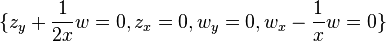
is obtained. It yields the general solution $z=C_1-C_2x, w=2C_2y$ with two undetermined constants $C_1$ and $C_2$ .

Janet's algorithm has been implemented in Maple

^[8] an implementation is also available on the website www.alltypes.de.

Application of Janet bases

The most important application of a Janet basis is its use for deciding the degree of indeterminacy of a system of linear homogeneous partial differential equations. The answer in the above Example 1 is that the system under consideration allows only the trivial solution. In the second Example 2 a two-dimensional solution space is obtained. In general, the answer may be more involved, there may be infinitely many free constants in the general solution; they may be obtained from the Loewy decomposition of the respective Janet basis.^[9] Furthermore, the Janet basis of a module allows to read off a Janet basis for the syzygy module ^[5]

References

↑ M. Janet, Les systèmes d'équations aux dérivées partielles, Journal de mathématiques pures et appliquées 8 ser., t. 3 (1920), pages 65–123.
↑ F. Schwarz, "Janet Bases for Symmetry Groups", in: Groebner Bases and Applications; Lecture Notes Series 251, London Mathematical Society, pages 221–234 (1998); B. Buchberger and F. Winkler, Edts.
↑ B. Buchberger, Ein algorithmisches Kriterium fuer die Loesbarkeit eines algebraischen Gleichungssystems, Aequ. Math. 4, 374–383(1970).
↑ F. Schwarz, Algorithmic Lie Theory for Solving Linear Ordinary Differential Equations, Chapman & Hall/CRC, 2007 Chapter 2.
1 2 W. Plesken, D. Robertz, Janet's approach to presentations and resolutions for polynomials and linear pdes, Archiv der Mathematik 84, page 22–37, 2005.
↑ T. Oaku, T. Shimoyama, A Groebner Basis Method for Modules over Rings of Differential Operators, Journal of Symbolic Computation 18, page 223–248, 1994.
↑ W. Adams, P. Loustaunau, An introduction to Groebner bases, American Mathematical Society, Providence, 1994.
↑ S. Zhang, Z. Li, An Implementation for the Algorithm of Janet bases of Linear Differential Ideals in the Maple System, Acta Mathematicae Applicatae Sinica, English Series, 20, page 605-616 (2004)
↑ F. Schwarz, Loewy Decomposition of Linear Differential Equations, Springer, 2013.

This article is issued from Wikipedia - version of the 5/13/2016. The text is available under the Creative Commons Attribution/Share Alike but additional terms may apply for the media files.