German tank problem

During World War II, production of German tanks such as the Panther was accurately estimated by Allied intelligence using statistical methods

In the statistical theory of estimation, the German tank problem involves estimating the maximum of a discrete uniform distribution from sampling without replacement. It is named from its application in World War II to the estimation of the number of German tanks.

This analysis shows the approach that was used and illustrates the difference between frequentist inference and Bayesian inference.

Estimating the population maximum based on a single sample yields divergent results, while the estimation based on multiple samples is an instructive practical estimation question whose answer is simple but not obvious.

Example

Graphs of estimated population size, N for number of samples, k and largest sample serial number, m using frequentist (dotted lines) and Bayesian analysis (solid line shows mean and shading shows range from minimum possible value to mean plus 1 standard deviation). The example shows if 4 tanks are observed and the highest serial number is 60, frequentist analysis predicts N = 74 whereas Bayesian analysis predicts a mean of 88.5 and standard deviation of 138.72 − 88.5 = 50.22, and a minimum of 60 tanks. In the SVG file, hover over a graph to highlight it.

Suppose k = 4 tanks with serial numbers 19, 40, 42 and 60 are captured. The maximal observed serial number, m = 60. The unknown total number of tanks is called N.

The formula for estimating the total number of tanks suggested by the frequentist approach outlined below is

N\approx m+{\frac {m}{k}}-1=74,

whereas the Bayesian analysis below yields (primarily) a probability mass function for the number of tanks

\Pr(N=n)={\begin{cases}0&{\text{if }}n<m\\{\frac {k-1}{k}}{\frac {\binom {m-1}{k-1}}{\binom {n}{k}}}&{\text{if }}n\geq m\end{cases}},

from which we can estimate the number of tanks according to

{\begin{aligned}N&\approx \mu \pm \sigma =88.5\pm 50.22,\\\mu &=(m-1){\frac {k-1}{k-2}},\\\sigma &={\sqrt {\frac {(k-1)(m-1)(m-k+1)}{(k-3)(k-2)^{2}}}}.\end{aligned}}

This distribution has positive skewness, related to the fact that there are at least 60 tanks.

Historical problem

Panther tanks are loaded for transport to frontline units, 1943

During the course of the war, the Western Allies made sustained efforts to determine the extent of German production and approached this in two major ways: conventional intelligence gathering and statistical estimation. In many cases, statistical analysis substantially improved on conventional intelligence. In some cases, conventional intelligence was used in conjunction with statistical methods, as was the case in estimation of Panther tank production just prior to D-Day.

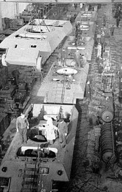
The allied command structure had thought the Panzer V (Panther) tanks seen in Italy, with their high velocity, long-barreled 75 mm/L70 guns, were unusual heavy tanks and would only be seen in northern France in small numbers, much the same way as the Tiger I was seen in Tunisia. The US Army was confident that the Sherman tank would continue to perform well, as it had versus the Panzer III and Panzer IV tanks in North Africa and Sicily.^{[N 1]} Shortly before D-Day, rumors indicated that large numbers of Panzer V tanks were being used.

To determine whether this was true, the Allies attempted to estimate the number of tanks being produced. To do this, they used the serial numbers on captured or destroyed tanks. The principal numbers used were gearbox numbers, as these fell in two unbroken sequences. Chassis and engine numbers were also used, though their use was more complicated. Various other components were used to cross-check the analysis. Similar analyses were done on tires, which were observed to be sequentially numbered (i.e., 1, 2, 3, ..., N).^[2]^{[lower-alpha 1]}^[3]^[4]

The analysis of tank wheels yielded an estimate for the number of wheel molds that were in use. A discussion with British road wheel makers then estimated the number of wheels that could be produced from this many molds, which yielded the number of tanks that were being produced each month. Analysis of wheels from two tanks (32 road wheels each, 64 road wheels total) yielded an estimate of 270 tanks produced in February 1944, substantially more than had previously been suspected.^[5]

German records after the war showed production for the month of February 1944 was 276.^[6]^{[N 2]} The statistical approach proved to be far more accurate than conventional intelligence methods, and the phrase "German tank problem" became accepted as a descriptor for this type of statistical analysis.

Estimating production was not the only use of this serial-number analysis. It was also used to understand German production more generally, including number of factories, relative importance of factories, length of supply chain (based on lag between production and use), changes in production, and use of resources such as rubber.

Specific data

According to conventional Allied intelligence estimates, the Germans were producing around 1,400 tanks a month between June 1940 and September 1942. Applying the formula below to the serial numbers of captured tanks, the number was calculated to be 256 a month. After the war, captured German production figures from the ministry of Albert Speer showed the actual number to be 255.^[3]

Estimates for some specific months are given as:^[7]

Month	Statistical estimate	Intelligence estimate	German records
June 1940	169	1,000	122
June 1941	244	1,550	271
August 1942	327	1,550	342

Similar analyses

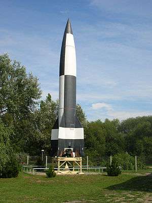
V-2 rocket production was accurately estimated by statistical methods

Similar serial-number analysis was used for other military equipment during World War II, most successfully for the V-2 rocket.^[8]

Factory markings on Soviet military equipment were analyzed during the Korean War, and by German intelligence during World War II.^[9]

In the 1980s, some Americans were given access to the production line of Israel's Merkava tanks. The production numbers were classified, but the tanks had serial numbers, allowing estimation of production.^[10]

The formula has been used in non-military contexts, for example to estimate the number of Commodore 64 computers built, where the result (12.5 million) matches the low-end estimates.^[11]

Countermeasures

To prevent serial-number analysis, serial numbers can be excluded, or usable auxiliary information reduced. Alternatively, serial numbers that resist cryptanalysis can be used, most effectively by randomly choosing numbers without replacement from a list that is much larger than the number of objects produced (compare the one-time pad), or produce random numbers and check them against the list of already assigned numbers; collisions are likely to occur unless the number of digits possible is more than twice the number of digits in the number of objects produced (where the serial number can be in any base); see birthday problem.^{[lower-alpha 2]} For this, a cryptographically secure pseudorandom number generator may be used. All these methods require a lookup table (or breaking the cypher) to back out from serial number to production order, which complicates use of serial numbers: a range of serial numbers cannot be recalled, for instance, but each must be looked up individually, or a list generated.

Alternatively, sequential serial numbers can be encrypted with a simple substitution cipher, which allows easy decoding, but is also easily broken by a known-plaintext attack: even if starting from an arbitrary point, the plaintext has a pattern (namely, numbers are in sequence). One example is given in Ken Follett's novel "Code to Zero", where the encryption of the Jupiter-C rocket serial numbers is described as:

H	U	N	T	S	V	I	L	E	X
1	2	3	4	5	6	7	8	9	0

The code word here is Huntsville (with repeated letters omitted) to get a 10-letter key. The rocket number 13 was therefore "HN", or the rocket number 24 was "UT".

Strong encryption of serial numbers without expanding them can be achieved with format-preserving encryption. Instead of storing a truly random permutation on the set of all possible serial numbers in a large table, such algorithms will derive a pseudo-random permutation from a secret key. Security can then be defined as the pseudo-random permutation being indistinguishable from a truly random permutation to an attacker who doesn't know the key.

Frequentist analysis

Minimum-variance unbiased estimator

For point estimation (estimating a single value for the total, ${\hat {N}}$ ), the minimum-variance unbiased estimator (MVUE, or UMVU estimator) is given by:^{[lower-alpha 3]}

{\hat {N}}=m\left(1+k^{-1}\right)-1,

where m is the largest serial number observed (sample maximum) and k is the number of tanks observed (sample size).^[10]^[12]^[13] Note that once a serial number has been observed, it is no longer in the pool and will not be observed again.

This has a variance^[10]

\operatorname {Var} ({\hat {N}})={\frac {1}{k}}{\frac {(N-k)(N+1)}{(k+2)}}\approx {\frac {N^{2}}{k^{2}}}{\text{ for small samples }}k\ll N,

so the standard deviation is approximately N/k, the average size of the gap between samples; compare m/k above.

Intuition

The formula may be understood intuitively as the sample maximum plus the average gap between observations in the sample, the sample maximum being chosen as the initial estimator, due to being the maximum likelihood estimator,^{[lower-alpha 4]} with the gap being added to compensate for the negative bias of the sample maximum as an estimator for the population maximum,^{[lower-alpha 5]} and written as

{\hat {N}}=m+{\frac {m-k}{k}}=m+mk^{-1}-1=m\left(1+k^{-1}\right)-1.

This can be visualized by imagining that the samples are evenly spaced throughout the range, with additional samples just outside the range at 0 and N + 1. If starting with an initial gap between 0 and the lowest sample (sample minimum), the average gap between samples is $(m-k)/k$ ; the $-k$ being because the samples themselves are not counted in computing the gap between samples.^{[lower-alpha 6]}

This philosophy is formalized and generalized in the method of maximum spacing estimation; a similar heuristic is used for plotting position in a Q–Q plot, plotting sample points at $k / (n + 1)$ , which is evenly on the uniform distribution, with a gap at the end.

Derivation

For any integer m such that k ≤ m ≤ N, the probability that the sample maximum will be equal to m is given by ${\big (}{\tbinom {m}{k}}-{\tbinom {m-1}{k}}{\big )}{\big /}{\tbinom {N}{k}}={\tbinom {m-1}{k-1}}{\big /}{\tbinom {N}{k}}$ , where ${\tbinom {\cdot }{\cdot }}$ is the binomial coefficient.

Given the total number N and the sample size k, the expected value of the sample maximum is

{\begin{aligned}\mu &=E(m)=\sum _{m=k}^{N}m{\frac {\tbinom {m-1}{k-1}}{\tbinom {N}{k}}}={\frac {k(N+1)}{k+1}}.\end{aligned}}

From this, the unknown quantity N can be expressed in terms of expectation and sample size as

{\begin{aligned}N&=\mu \left(1+k^{-1}\right)-1.\end{aligned}}

By linearity of the expectation, it is obtained that

{\begin{aligned}\mu \left(1+k^{-1}\right)-1&=E\left[m\left(1+k^{-1}\right)-1\right],\end{aligned}}

and so an unbiased estimator of N is obtained by replacing the expectation with the observation, so that

{\begin{aligned}{\hat {N}}&=m\left(1+k^{-1}\right)-1.\end{aligned}}

To show that this is the UMVU estimator:

First, show that the sample maximum is a sufficient statistic for the population maximum, using a method similar to that detailed at sufficiency: uniform distribution (but for the German tank problem we must exclude the outcomes in which a serial number occurs twice in the sample).
Next, show that it is a complete statistic.
Then the Lehmann–Scheffé theorem states that the sample maximum, corrected for bias as above to be unbiased, is the UMVU estimator.

Confidence intervals

Instead of, or in addition to, point estimation, interval estimation can be carried out, such as confidence intervals. These are easily computed, based on the observation that the probability that k samples will fall in an interval covering p of the range (0 ≤ p ≤ 1) is p^k (assuming in this section that draws are with replacement, to simplify computations; if draws are without replacement, this overstates the likelihood, and intervals will be overly conservative).

Thus the sampling distribution of the quantile of the sample maximum is the graph x^1/k from 0 to 1: the p-th to q-th quantile of the sample maximum m are the interval [p^1/kN, q^1/kN]. Inverting this yields the corresponding confidence interval for the population maximum of [m/q^1/k, m/p^1/k].

For example, taking the symmetric 95% interval p = 2.5% and q = 97.5% for k = 5 yields 0.025^1/5 ≈ 0.48, 0.975^1/5 ≈ 0.995, so the confidence interval is approximately [1.005m, 2.08m]. The lower bound is very close to m, thus more informative is the asymmetric confidence interval from p = 5% to 100%; for k = 5 this yields 0.05^1/5 ≈ 0.55 and the interval [m, 1.82m].

More generally, the (downward biased) 95% confidence interval is [m, m/0.05^1/k] = [m, m·20^1/k]. For a range of k values, with the UMVU point estimator (plus 1 for legibility) for reference, this yields:

k	point estimate	confidence interval
1	2m	[m, 20m]
2	1.5m	[m, 4.5m]
5	1.2m	[m, 1.82m]
10	1.1m	[m, 1.35m]
20	1.05m	[m, 1.16m]

Immediate observations are:

For small sample sizes, the confidence interval is very wide, reflecting great uncertainty in the estimate.
The range shrinks rapidly, reflecting the exponentially decaying likelihood that all samples will be significantly below the maximum.
The confidence interval exhibits positive skew, as N can never be below the sample maximum, but can potentially be arbitrarily high above it.

Note that m/k cannot be used naively (or rather (m + m/k − 1)/k) as an estimate of the standard error SE, as the standard error of an estimator is based on the population maximum (a parameter), and using an estimate to estimate the error in that very estimate is circular reasoning.

In some fields, notably futurology, estimation of confidence intervals in this way, based on a single sample – considering it as a randomly sampled quantile (by mediocrity principle) – is known as the Copernican principle. This is particularly applied to estimate lifetimes based on current age, notably in the doomsday argument, which applies it to estimate the expected survival time of the human race.

Bayesian analysis

The Bayesian approach to the German tank problem is to consider the credibility $\scriptstyle (N=n\mid M=m,K=k)$ that the number of enemy tanks $\scriptstyle N$ is equal to the number $\scriptstyle n$ , when the number of observed tanks, $\scriptstyle K$ is equal to the number $\scriptstyle k$ , and the maximum serial number $\scriptstyle M$ is equal to the number $\scriptstyle m$ . The answer to this problem depends on the choice of prior for $\scriptstyle N$ . One can proceed using a proper prior, e.g., the Poisson or Negative Binomial distribution, where closed formula for the posterior mean and posterior variance can be obtained.^[14] An alternative is to proceed using direct calculations as shown below.

For brevity, in what follows, $\scriptstyle (N=n\mid M=m,K=k)$ is written $\scriptstyle (n\mid m,k)$

Conditional probability

The rule for conditional probability gives

(n\mid m,k)(m\mid k)=(m\mid n,k)(n\mid k)=(m,n\mid k)

Probability of M knowing N and K

The expression

(m\mid n,k)=(M=m\mid N=n,K=k)

is the conditional probability that the maximum serial number observed, M, is equal to m, when the number of enemy tanks, N, is known to be equal to n, and the number of enemy tanks observed, K, is known to be equal to k.

It is

(m\mid n,k)={\binom {m-1}{k-1}}{\binom {n}{k}}^{-1}[k\leq m][m\leq n]

where $\scriptstyle {\binom {n}{k}}$ is a binomial coefficient and $\scriptstyle [k\leq n]$ is an Iverson bracket.

Probability of M knowing only K

The expression $\scriptstyle (m\mid k)=(M=m\mid K=k)$ is the probability that the maximum serial number is equal to m once k tanks have been observed but before the serial numbers have actually been observed.

The expression $\scriptstyle (m\mid k)$ can be re-written in terms of the other quantities by marginalizing over all possible $\scriptstyle n$ .

{\begin{aligned}(m\mid k)&=(m\mid k)\cdot 1\\&=(m\mid k){\sum _{n=0}^{\infty }(n\mid m,k)}\\&=(m\mid k){\sum _{n=0}^{\infty }(m\mid n,k){\frac {(n\mid k)}{(m\mid k)}}}\\&=\sum _{n=0}^{\infty }(m\mid n,k)(n\mid k)\end{aligned}}

Credibility of N knowing only K

The expression

(n\mid k)=(N=n\mid K=k)

is the credibility that the total number of tanks, N, is equal to n when the number K tanks observed is known to be k, but before the serial numbers have been observed. Assume that it is some discrete uniform distribution

(n\mid k)=(\Omega -k)^{-1}[k\leq n][n<\Omega ]

The upper limit $\Omega$ must be finite, because the function

f(n)=\lim _{\Omega \rightarrow \infty }(\Omega -k)^{-1}[k\leq n][n<\Omega ]=0

is not a mass distribution function.

Credibility of N knowing M and K

(n\mid m,k)=(m\mid n,k)\left(\sum _{n=m}^{\Omega -1}(m\mid n,k)\right)^{-1}[m\leq n][n<\Omega ]

If k ≥ 2, then $\scriptstyle \sum _{n=m}^{\infty }(m\mid n,k)<\infty$ , and the unwelcome variable $\scriptstyle \Omega$ disappears from the expression.

(n\mid m,k)=(m\mid n,k)\left(\sum _{n=m}^{\infty }(m\mid n,k)\right)^{-1}[m\leq n]

For k ≥ 1 the mode of the distribution of the number of enemy tanks is m.

For k ≥ 2, the credibility that the number of enemy tanks is equal to $n$ , is

(N=n\mid m,k)=(k-1){\binom {m-1}{k-1}}k^{-1}{\binom {n}{k}}^{-1}[m\leq n]

The credibility that the number of enemy tanks, N, is greater than n, is

(N>n\mid m,k)={\begin{cases}1&{\text{if }}n<m\\{\frac {\binom {m-1}{k-1}}{\binom {n}{k-1}}}&{\text{if }}n\geq m\end{cases}}

Mean value and standard deviation

For k ≥ 3, N has the finite mean value:

(m-1)(k-1)(k-2)^{-1}

For k ≥ 4, N has the finite standard deviation:

(k-1)^{1/2}(k-2)^{-1}(k-3)^{-1/2}(m-1)^{1/2}(m+1-k)^{1/2}

These formulas are derived below.

Summation formula

The following binomial coefficient identity is used below for simplifying series relating to the German Tank Problem.

\sum _{n=m}^{\infty }{\frac {1}{\binom {n}{k}}}={\frac {k}{k-1}}{\frac {1}{\binom {m-1}{k-1}}}

This sum formula is somewhat analogous to the integral formula

\int _{n=m}^{\infty }{\frac {dn}{n^{k}}}={\frac {1}{k-1}}{\frac {1}{m^{k-1}}}

These formulas apply for k > 1.

One tank

Observing one tank randomly out of a population of n tanks gives the serial number m with probability 1/n for m ≤ n, and zero probability for m > n. Using Iverson bracket notation this is written

(M=m\mid N=n,K=1)=(m\mid n)={\frac {[m\leq n]}{n}}

This is the conditional probability mass distribution function of $\scriptstyle m$ .

When considered a function of n for fixed m this is a likelihood function.

{\mathcal {L}}(n)={\frac {[n\geq m]}{n}}

The maximum likelihood estimate for the total number of tanks is N₀ = m.

The total likelihood is infinite, being a tail of the harmonic series.

\sum _{n}{\mathcal {L}}(n)=\sum _{n=m}^{\infty }{\frac {1}{n}}=\infty

but

{\begin{aligned}\sum _{n}{\mathcal {L}}(n)[n<\Omega ]&=\sum _{n=m}^{\Omega -1}{\frac {1}{n}}\\&=H_{\Omega -1}-H_{m-1}\end{aligned}}

where $H_{n}$ is the harmonic number.

The credibility mass distribution function depends on the prior limit $\scriptstyle \Omega$ :

{\begin{aligned}&(N=n\mid M=m,K=1)\\={}&(n\mid m)={\frac {[m\leq n]}{n}}{\frac {[n<\Omega ]}{H_{\Omega -1}-H_{m-1}}}\end{aligned}}

The mean value of $\scriptstyle N$ is

{\begin{aligned}\sum _{n}n\cdot (n\mid m)&=\sum _{n=m}^{\Omega -1}{\frac {1}{H_{\Omega -1}-H_{m-1}}}\\&={\frac {\Omega -m}{H_{\Omega -1}-H_{m-1}}}\\&\approx {\frac {\Omega -m}{\log \left({\frac {\Omega -1}{m-1}}\right)}}\end{aligned}}

Two tanks

If two tanks rather than one are observed, then the probability that the larger of the observed two serial numbers is equal to m, is

(M=m\mid N=n,K=2)=(m\mid n)=[m\leq n]{\frac {m-1}{\binom {n}{2}}}

When considered a function of n for fixed m this is a likelihood function

{\mathcal {L}}(n)=[n\geq m]{\frac {m-1}{\binom {n}{2}}}

The total likelihood is

{\begin{aligned}\sum _{n}{\mathcal {L}}(n)&={\frac {m-1}{1}}\sum _{n=m}^{\infty }{\frac {1}{\binom {n}{2}}}\\&={\frac {m-1}{1}}\cdot {\frac {2}{2-1}}\cdot {\frac {1}{\binom {m-1}{2-1}}}\\&=2\end{aligned}}

and the credibility mass distribution function is

{\begin{aligned}&(N=n\mid M=m,K=2)\\={}&(n\mid m)\\={}&{\frac {{\mathcal {L}}(n)}{\sum _{n}{\mathcal {L}}(n)}}\\={}&[n\geq m]{\frac {m-1}{n(n-1)}}\end{aligned}}

The median $\scriptstyle {\tilde {N}}$ satisfies

\sum _{n}[n\geq {\tilde {N}}](n\mid m)={\frac {1}{2}}

{\frac {m-1}{{\tilde {N}}-1}}={\frac {1}{2}}

and so the median is

{\tilde {N}}=2m-1

but the mean value of N is infinite

\mu =\sum _{n}n\cdot (n\mid m)={\frac {m-1}{1}}\sum _{n=m}^{\infty }{\frac {1}{n-1}}=\infty

Many tanks

Credibility mass distribution function

The conditional probability that the largest of k observations taken from the serial numbers {1,...,n}, is equal to m, is

{\begin{aligned}&(M=m\mid N=n,K=k\geq 2)\\={}&(m\mid n,k)\\={}&[m\leq n]{\frac {\binom {m-1}{k-1}}{\binom {n}{k}}}\end{aligned}}

The likelihood function of n is the same expression

{\mathcal {L}}(n)=[n\geq m]{\frac {\binom {m-1}{k-1}}{\binom {n}{k}}}

The total likelihood is finite for k ≥ 2:

{\begin{aligned}\sum _{n}{\mathcal {L}}(n)&={\frac {\binom {m-1}{k-1}}{1}}\sum _{n=m}^{\infty }{1 \over {\binom {n}{k}}}\\&={\frac {\binom {m-1}{k-1}}{1}}\cdot {\frac {k}{k-1}}\cdot {\frac {1}{\binom {m-1}{k-1}}}\\&={\frac {k}{k-1}}\end{aligned}}

The credibility mass distribution function is

{\begin{aligned}&(N=n\mid M=m,K=k\geq 2)=(n\mid m,k)\\={}&{\frac {{\mathcal {L}}(n)}{\sum _{n}{\mathcal {L}}(n)}}\\={}&[n\geq m]{\frac {k-1}{k}}{\frac {\binom {m-1}{k-1}}{\binom {n}{k}}}\\={}&[n\geq m]{\frac {m-1}{n}}{\frac {\binom {m-2}{k-2}}{\binom {n-1}{k-1}}}\\={}&[n\geq m]{\frac {m-1}{n}}{\frac {m-2}{n-1}}{\frac {k-1}{k-2}}{\frac {\binom {m-3}{k-3}}{\binom {n-2}{k-2}}}\end{aligned}}

The complementary cumulative distribution function is the credibility that N > x

{\begin{aligned}&(N>x\mid M=m,K=k)\\={}&{\begin{cases}1&{\text{if }}x<m\\\sum _{n=x+1}^{\infty }(n\mid m,k)&{\text{if }}x\geq m\end{cases}}\\={}&[x<m]+[x\geq m]\sum _{n=x+1}^{\infty }{\frac {k-1}{k}}{\frac {\binom {m-1}{k-1}}{\binom {N}{k}}}\\={}&[x<m]+[x\geq m]{\frac {k-1}{k}}{\frac {\binom {m-1}{k-1}}{1}}\sum _{n=x+1}^{\infty }{\frac {1}{\binom {n}{k}}}\\={}&[x<m]+[x\geq m]{\frac {k-1}{k}}{\frac {\binom {m-1}{k-1}}{1}}\cdot {\frac {k}{k-1}}{\frac {1}{\binom {x}{k-1}}}\\={}&[x<m]+[x\geq m]{\frac {\binom {m-1}{k-1}}{\binom {x}{k-1}}}\end{aligned}}

The cumulative distribution function is the credibility that N ≤ x

{\begin{aligned}&(N\leq x\mid M=m,K=k)\\={}&1-(N>x\mid M=m,K=k)\\={}&[x\geq m]\left(1-{\frac {\binom {m-1}{k-1}}{\binom {x}{k-1}}}\right)\end{aligned}}

Order of magnitude

The order of magnitude of the number of enemy tanks is

{\begin{aligned}\mu &=\sum _{n}n\cdot (N=n\mid M=m,K=k)\\&=\sum _{n}n[n\geq m]{\frac {m-1}{n}}{\frac {\binom {m-2}{k-2}}{\binom {n-1}{k-1}}}\\&={\frac {m-1}{1}}{\frac {\binom {m-2}{k-2}}{1}}\sum _{n=m}^{\infty }{\frac {1}{\binom {n-1}{k-1}}}\\&={\frac {m-1}{1}}{\frac {\binom {m-2}{k-2}}{1}}\cdot {\frac {k-1}{k-2}}{\frac {1}{\binom {m-2}{k-2}}}\\&={\frac {m-1}{1}}{\frac {k-1}{k-2}}\end{aligned}}

Statistical uncertainty

The statistical uncertainty is the standard deviation σ, satisfying the equation

\sigma ^{2}+\mu ^{2}=\sum _{n}n^{2}\cdot (N=n\mid M=m,K=k)

{\begin{aligned}\sigma ^{2}+\mu ^{2}-\mu &=\sum _{n}n(n-1)\cdot (N=n\mid M=m,K=k)\\&=\sum _{n=m}^{\infty }n(n-1){\frac {m-1}{n}}{\frac {m-2}{n-1}}{\frac {k-1}{k-2}}{\frac {\binom {m-3}{k-3}}{\binom {n-2}{k-2}}}\\&={\frac {m-1}{1}}{\frac {m-2}{1}}{\frac {k-1}{k-2}}\cdot {\frac {\binom {m-3}{k-3}}{1}}\sum _{n=m}^{\infty }{\frac {1}{\binom {n-2}{k-2}}}\\&={\frac {m-1}{1}}{\frac {m-2}{1}}{\frac {k-1}{k-2}}{\frac {\binom {m-3}{k-3}}{1}}{\frac {k-2}{k-3}}{\frac {1}{\binom {m-3}{k-3}}}\\&={\frac {m-1}{1}}{\frac {m-2}{1}}{\frac {k-1}{k-3}}\\&\end{aligned}}

and

{\begin{aligned}\sigma &={\sqrt {{\frac {m-1}{1}}{\frac {m-2}{1}}{\frac {k-1}{k-3}}+\mu -\mu ^{2}}}\\&={\sqrt {\frac {(k-1)(m-1)(m-k+1)}{(k-3)(k-2)^{2}}}}\\&\end{aligned}}

The variance-to-mean ratio is simply

{\frac {\sigma ^{2}}{\mu }}={\frac {m-k+1}{(k-3)(k-2)}}

References

Notes

↑ An Armored Ground Forces policy statement of November 1943 concluded: "The recommendation of a limited proportion of tanks carrying a 90 mm gun is not concurred in for the following reasons: The M4 tank has been hailed widely as the best tank of the battlefield today. ... There appears to be no fear on the part of our forces of the German Mark VI (Tiger) tank. There can be no basis for the T26 tank other than the conception of a tank-vs.-tank duel – which is believed to be unsound and unnecessary."^[1]
↑ Ruggles & Brodie is largely a practical analysis and summary, not a mathematical one – the estimation problem is only mentioned in footnote 3 on page 82, where they estimate the maximum as "sample maximum + average gap".

↑ The lower bound was unknown, but to simplify the discussion, this detail is generally omitted, taking the lower bound as known to be 1.
↑ As discussed in birthday attack, one can expect a collision after 1.25√H numbers, if choosing from H possible outputs. This square root corresponds to half the digits. For example, the square root of a number with 100 digits is approximately a number with 50 digits in any base.
↑ In a continuous distribution, there is no −1 term.
↑ Given a particular set of observations, this set is most likely to occur if the population maximum is the sample maximum, not a higher value (it cannot be lower).
↑ The sample maximum is never more than the population maximum, but can be less, hence it is a biased estimator: it will tend to underestimate the population maximum.
↑ For example, the gap between 2 and 7 is (7 − 2) − 1 = 4, consisting of 3, 4, 5, and 6.

Citations

↑ AGF policy statement. Chief of staff AGF. November 1943. MHI
↑ Ruggles & Brodie 1947, p. ?.
1 2 "Gavyn Davies does the maths – How a statistical formula won the war". The Guardian. 20 July 2006. Retrieved 6 July 2014.
↑ Matthews, Robert (23 May 1998), "Data sleuths go to war, sidebar in feature "Hidden truths"", New Scientist, archived from the original on 18 April 2001
↑ Bob Carruthers (2012-03-01). Panther V in Combat. Coda Books Ltd. pp. 94–. ISBN 978-1-908538-15-4.
↑ Ruggles & Brodie 1947, pp. 82–83.
↑ Ruggles & Brodie 1947, p. 89.
↑ Ruggles & Brodie 1947, pp. 90–91.
↑ Volz 2008.
1 2 3 Johnson 1994.
↑ "How many Commodore 64 computers were really sold?". pagetable.com. 1 February 2011. Archived from the original on 6 March 2016. Retrieved 6 July 2014.
↑ Johnson, Roger (2006), "Estimating the Size of a Population" (PDF), Getting the Best from Teaching Statistics
↑ Joyce, Smart. "German Tank Problem". Logan High School. Archived from the original on 2012-04-24. Retrieved 8 July 2014.
↑ Höhle, M.; Held, L. (2006). "Bayesian Estimation of the Size of a Population" (PDF). Technical Report SFB 386, No. 399, Department of Statistics, University of Munich. Retrieved 2016-04-17.

Bibliography

Goodman, L. A. (1954). "Some Practical Techniques in Serial Number Analysis". Journal of the American Statistical Association. American Statistical Association. 49 (265): 97–112. doi:10.2307/2281038. JSTOR 2281038.
Höhle, M.; Held, Leonhard (2006). "Bayesian Estimation of the Size of a Population" (PDF). Technical Report, SFB 386, No. 399, Department of Statistics, University of Munich. Retrieved 2016-04-17.
Johnson, R. W. (Summer 1994). "Estimating the Size of a Population". Teaching Statistics. 16 (2): 50–52. doi:10.1111/j.1467-9639.1994.tb00688.x.
Ruggles, R.; Brodie, H. (1947). "An Empirical Approach to Economic Intelligence in World War II". Journal of the American Statistical Association. 42 (237): 72. doi:10.1080/01621459.1947.10501915. JSTOR 2280189.
Volz, A. G. (July 2008). "A Soviet Estimate of German Tank Production". The Journal of Slavic Military Studies. 21 (3): 588–590. doi:10.1080/13518040802313902.

Probability distributions

List

Discrete univariate with finite support	Benford Bernoulli beta-binomial binomial categorical hypergeometric Poisson binomial Rademacher discrete uniform Zipf Zipf–Mandelbrot

Discrete univariate with infinite support	beta negative binomial Borel Conway–Maxwell–Poisson discrete phase-type Delaporte extended negative binomial Gauss–Kuzmin geometric logarithmic negative binomial parabolic fractal Poisson Skellam Yule–Simon zeta

Continuous univariate supported on a bounded interval	arcsine ARGUS Balding–Nichols Bates beta beta rectangular Irwin–Hall Kumaraswamy logit-normal noncentral beta raised cosine reciprocal triangular U-quadratic uniform Wigner semicircle

Continuous univariate supported on a semi-infinite interval	Benini Benktander 1st kind Benktander 2nd kind beta prime Burr chi-squared chi Dagum Davis exponential-logarithmic Erlang exponential F folded normal Flory–Schulz Fréchet gamma gamma/Gompertz generalized inverse Gaussian Gompertz half-logistic half-normal Hotelling's T-squared hyper-Erlang hyperexponential hypoexponential inverse chi-squared scaled inverse chi-squared inverse Gaussian inverse gamma Kolmogorov Lévy log-Cauchy log-Laplace log-logistic log-normal Lomax matrix-exponential Maxwell–Boltzmann Maxwell–Jüttner Mittag-Leffler Nakagami noncentral chi-squared Pareto phase-type poly-Weibull Rayleigh relativistic Breit–Wigner Rice shifted Gompertz truncated normal type-2 Gumbel Weibull Discrete Weibull Wilks's lambda

Continuous univariate supported on the whole real line	Cauchy exponential power Fisher's z Gaussian q generalized normal generalized hyperbolic geometric stable Gumbel Holtsmark hyperbolic secant Johnson's S_U Landau Laplace asymmetric Laplace logistic noncentral t normal (Gaussian) normal-inverse Gaussian skew normal slash stable Student's t type-1 Gumbel Tracy–Widom variance-gamma Voigt

Continuous univariate with support whose type varies	generalized extreme value generalized Pareto Tukey lambda q-Gaussian q-exponential q-Weibull shifted log-logistic

Mixed continuous-discrete univariate	rectified Gaussian

Multivariate (joint)	Discrete Ewens multinomial Dirichlet-multinomial negative multinomial Continuous Dirichlet generalized Dirichlet multivariate normal multivariate stable multivariate t normal-inverse-gamma normal-gamma Matrix-valued inverse matrix gamma inverse-Wishart matrix normal matrix t matrix gamma normal-inverse-Wishart normal-Wishart Wishart

Directional	Univariate (circular) directional Circular uniform univariate von Mises wrapped normal wrapped Cauchy wrapped exponential wrapped asymmetric Laplace wrapped Lévy Bivariate (spherical) Kent Bivariate (toroidal) bivariate von Mises Multivariate von Mises–Fisher Bingham

Degenerate and singular	Degenerate Dirac delta function Singular Cantor

Families	Circular compound Poisson elliptical exponential natural exponential location-scale maximum entropy mixture Pearson Tweedie wrapped

This article is issued from Wikipedia - version of the 11/18/2016. The text is available under the Creative Commons Attribution/Share Alike but additional terms may apply for the media files.