Geopotential model
In geophysics, a geopotential model is the theoretical analysis of measuring and calculating the effects of Earth's gravitational field.
Newton's law
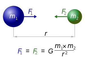
Newton's law of universal gravitation states that the gravitational force F acting between two point masses m1 and m2 with centre of mass separation r is given by

where G is the gravitational constant and r̂ is the radial unit vector. For an object of continuous mass distribution, each mass element dm can be treated as a point mass, so the volume integral over the extent of the object gives:
-
(1)

with corresponding gravitational potential
-
(2)

where ρ = ρ(x, y, z) is the mass density at the volume element and of the direction from the volume element to the point mass.
The case of a homogeneous sphere
In the special case of a sphere with a spherically symmetric mass density then ρ = ρ(s), i.e. density depends only on the radial distance

These integrals can be evaluated analytically. This is the shell theorem saying that in this case:
-
(3)

with corresponding potential
-
(4)

where M = ∫Vρ(s)dxdydz is the total mass of the sphere.
The deviations of Earth's gravitational field from that of a homogeneous sphere
In reality, Earth is not exactly spherical, mainly because of its rotation around the polar axis that makes its shape slightly oblate. If this shape would have been perfectly known together with the exact mass density ρ = ρ(x, y, z) the integrals (1) and (2) could have been evaluated with numerical methods to find a more accurate model for Earth's gravitational field, but the situation is in fact the opposite. By observing the orbits of spacecraft and the Moon, Earth's gravitational field can be determined quite accurately and the best estimate of Earth's mass is obtained by dividing the product GM as determined from the analysis of spacecraft orbit with a value for G determined to a lower relative accuracy using other physical methods.
From the defining equations (1) and (2) it is clear (taking the partial derivatives of the integrand) that outside the body in empty space the following differential equations are valid for the field caused by the body:
-
(5)

-
(6)

Functions of the form where (r, θ, φ) are the spherical coordinates which satisfy the partial differential equation (6) (the Laplace equation) are called spherical harmonic function.

They take the forms:
-
(7)

where spherical coordinates (r, θ, φ) are used, given here in terms of cartesian (x, y, z) for reference:
-
(8)

also P0n are the Legendre polynomials and Pmn for 1 ≤ m ≤ n are the associated Legendre functions.
The first spherical harmonics with n = 0,1,2,3 are presented in the table below.
n Spherical harmonics 0 1 2 3


The model for Earth's gravitational potential is a sum
-
(9)

where and the coordinates (8) are relative the standard geodetic reference system extended into space with origin in the center of the reference ellipsoid and with z-axis in the direction of the polar axis.

The zonal terms refer to terms of the form:

and the tesseral terms terms refer to terms of the form:


The zonal and tesseral terms for n = 1 are left out in (9).
The different coefficients Jn, Cnm, Snm, are then given the values for which the best possible agreement between the computed and the observed spacecraft orbits is obtained.
As P0n(x) = −P0n(−x) non-zero coefficients Jn for odd n correspond to a lack of symmetry "north–south" relative the equatorial plane for the mass distribution of Earth. Non-zero coefficients Cnm, Snm correspond to a lack of rotational symmetry around the polar axis for the mass distribution of Earth, i.e. to a "tri-axiality" of Earth.
For large values of n the coefficients above (that are divided by r(n + 1) in (9)) take very large values when for example kilometers and seconds are used as units. In the literature it is common to introduce some arbitrary "reference radius" R close to Earth's radius and to work with the dimensionless coefficients


and to write the potential as
-
(10)

The dominating term (after the term −μ/r) in (9) is the "J2 term":

Relative the coordinate system
-
(11)

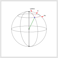

illustrated in figure 1 the components of the force caused by the "J2 term" are
-
(12)

In the rectangular coordinate system (x, y, z) with unit vectors (x̂ ŷ ẑ) the force components are:
-
(13)

The components of the force corresponding to the "J3 term"

are
-
(14)

and
-
(15)

The exact numerical values for the coefficients deviate (somewhat) between different Earth models but for the lowest coefficients they all agree almost exactly.
For JGM-3 the values are:
- μ = 398600.440 km3⋅s−2
- J2 = 1.7555 × 10¹⁰ km5⋅s−2
- J3 = −2.619 × 10¹¹ km6⋅s−2
With a "reference radius" R of 6378.1363 km corresponding dimensionless parameters are


For example, at a radius of 6600 km (about 200 km above Earth's surface) J3/(J2r) is about 0.002, i.e the correction to the "J2 force" from the "J3 term" is in the order of 2 permille. The negative value of J3 implies that for a point mass in Earth's equatorial plane the gravitational force is tilted slightly towards the south due to the lack of symmetry for the mass distribution of Earth's "north–south".
Recursive algorithms used for the numerical propagation of spacecraft orbits
Spacecraft orbits are computed by the numerical integration of the equation of motion. For this the gravitational force, i.e. the gradient of the potential, must be computed. Efficient recursive algorithms have been designed to compute the gravitational force for any and and such algorithms are used in standard orbit propagation software.


Available models
The earliest Earth models in general use by NASA and ESRO/ESA were the "Goddard Earth Models" developed by Goddard Space Flight Center denoted "GEM-1", "GEM-2", "GEM-3", and so on. Later the "Joint Earth Gravity Models" denoted "JGM-1", "JGM-2", "JGM-3" developed by Goddard Space Flight Center in cooperation with universities and private companies became available. The newer models generally provided higher order terms than their precursors. The EGM96 uses Nz = Nt = 360 resulting in 130317 coefficients.
For a normal Earth satellite for which an orbit determination/prediction accuracy of a few meters the "JGM-3" truncated to Nz = Nt = 36 (1365 coefficients) is usually sufficient. Inaccuracies from the modeling of the air-drag and to a lesser extent the solar radiation pressure will exceed the inaccuracies caused by the gravitation modeling errors.
Spherical harmonics
The following is a compact account of the spherical harmonics used to model Earth's gravitational field. The spherical harmonics are derived from the approach of looking for harmonic functions of the form
-
(16)
where (r, θ, φ) are the spherical coordinates defined by the equations (8). By straightforward calculations one gets that for any function f
-
(17)

Introducing the expression (16) in (17) one gets that
-
(18)

As the term

only depends on the variable and the sum


only depends on the variables θ and φ. One gets that φ is harmonic if and only if
-
(19)

and
-
(20)

for some constant

From (20) then follows that

The first two terms only depend on the variable and the third only on the variable .


From the definition of φ as a spherical coordinate it is clear that Φ(φ) must be periodic with the period 2π and one must therefore have that
-
(21)

and
-
(22)

for some integer m as the family of solutions to (21) then are
-
(23)

With the variable substitution

equation (22) takes the form
-
(24)

From (19) follows that in order to have a solution with


one must have that

If Pn(x) is a solution to the differential equation
-
(25)

one therefore has that the potential corresponding to m = 0

which is rotational symmetric around the z-axis is an harmonic function
If is a solution to the differential equation

-
(26)

with m ≥ 1 one has the potential
-
(27)

where a and b are arbitrary constants is a harmonic function that depends on φ and therefore is not rotational symmetric around the z-axis
The differential equation (25) is the Legendre differential equation for which the Legendre polynomials defined
-
(28)

are the solutions.
The arbitrary factor 1/(2nn!) is selected to make Pn(−1)=−1 and Pn(1) = 1 for odd n and Pn(−1) = Pn(1) = 1 for even n.
The first six Legendre polynomials are:
-
(29)

The solutions to differential equation (26) are the associated Legendre functions
-
(30)

One therefore has that

References
- El'Yasberg "Theory of flight of artificial earth satellites", Israel program for Scientific Translations (1967)
- Lerch, F.J., Wagner, C.A., Smith, D.E., Sandson, M.L., Brownd, J.E., Richardson, J.A.,"Gravitational Field Models for the Earth (GEM1&2)", Report X55372146, Goddard Space Flight Center, Greenbelt/Maryland, 1972
- Lerch, F.J., Wagner, C.A., Putney, M.L., Sandson, M.L., Brownd, J.E., Richardson, J.A., Taylor, W.A., "Gravitational Field Models GEM3 and 4" ,Report X59272476, Goddard Space Flight Center, Greenbelt/Maryland, 1972
- Lerch, F.J., Wagner, C.A., Richardson, J.A., Brownd, J.E., "Goddard Earth Models (5 and 6)", Report X92174145, Goddard Space Flight Center, Greenbelt/Maryland, 1974
- Lerch, F.J., Wagner, C.A., Klosko, S.M., Belott, R.P., Laubscher, R.E., Raylor, W.A., "Gravity Model Improvement Using Geos3 Altimetry (GEM10A and 10B)", 1978 Spring Annual Meeting of the American Geophysical Union, Miami, 1978
- Lerch, F.J., Klosko, S.M., Laubscher, R.E., Wagner, C.A., "Gravity Model Improvement Using Geos3 (GEM9 and 10)", Journal of Geophysical Research, Vol. 84, B8, p. 3897-3916, 1979
- Lerch,F.J., Putney, B.H., Wagner, C.A., Klosko, S.M. ,"Goddard earth models for oceanographic applications (GEM 10B and 10C)", Marine-Geodesy, 5(2), p. 145-187, 1981
- Lerch, F.J., Klosko, S.M., Patel, G.B., "A Refined Gravity Model from Lageos (GEML2)", 'NASA Technical Memorandum 84986, Goddard Space Flight Center, Greenbelt/Maryland, 1983
- Lerch, F.J., Nerem, R.S., Putney, B.H., Felsentreger, T.L., Sanchez, B.V., Klosko, S.M., Patel, G.B., Williamson, R.G., Chinn, D.S., Chan, J.C., Rachlin, K.E., Chandler, N.L., McCarthy, J.J., Marshall, J.A., Luthcke, S.B., Pavlis, D.W., Robbins, J.W., Kapoor, S., Pavlis, E.C., " Geopotential Models of the Earth from Satellite Tracking, Altimeter and Surface Gravity Observations: GEMT3 and GEMT3S", NASA Technical Memorandum 104555, Goddard Space Flight Center , Greenbelt/Maryland, 1992
- Lerch, F.J., Nerem, R.S., Putney, B.H., Felsentreger, T.L., Sanchez, B.V., Marshall, J.A., Klosko, S.M., Patel, G.B., Williamson, R.G., Chinn, D.S., Chan, J.C., Rachlin, K.E., Chandler, N.L., McCarthy, J.J., Luthcke, S.B., Pavlis, N.K., Pavlis, D.E., Robbins, J.W., Kapoor, S., Pavlis, E.C., "A Geopotential Model from Satellite Tracking, Altimeter and Surface Gravity Data: GEMT3", Journal of Geophysical Research, Vol. 99, No. B2, p. 2815-2839, 1994
- Nerem, R.S., Lerch, F.J., Marshall, J.A., Pavlis, E.C., Putney, B.H., Tapley, B.D., Eanses, R.J., Ries, J.C., Schutz, B.E., Shum, C.K., Watkins, M.M., Klosko, S.M., Chan, J.C., Luthcke, S.B., Patel, G.B., Pavlis, N.K., Williamson, R.G., Rapp, R.H., Biancale, R., Nouel, F., "Gravity Model Developments for Topex/Poseidon: Joint Gravity Models 1 and 2", Journal of Geophysical Research, Vol. 99, No. C12, p. 24421-24447, 1994a
External links
- http://cddis.nasa.gov/lw13/docs/papers/sci_lemoine_1m.pdf
- http://geodesy.geology.ohio-state.edu/course/refpapers/Tapley_JGR_JGM3_96.pdf