Geodesic grid
_illustrated.png)
A geodesic grid is a technique used to model the surface of a sphere (such as the Earth) with a subdivided polyhedron, usually an icosahedron.
Introduction
A geodesic grid is a global Earth reference that uses cells or tiles to statistically represent data encoded to the area covered by the cell location. The focus of the discrete cells in a geodesic grid reference is different from that of a conventional lattice-based Earth reference where the focus is on a continuity of points used for addressing location and navigation.
In biodiversity science, geodesic grids are a global extension of local discrete grids that are staked out in field studies to ensure appropriate statistical sampling and larger multi-use grids deployed at regional and national levels to develop an aggregated understanding of biodiversity. These grids translate environmental and ecological monitoring data from multiple spatial and temporal scales into assessments of current ecological condition and forecasts of risks to our natural resources. A geodesic grid allows local to global assimilation of ecologically significant information at its own level of granularity.[1]
When modeling the weather, ocean circulation, or the climate, partial differential equations are used to describe the evolution of these systems over time. Because computer programs are used to build and work with these complex models, approximations need to be formulated into easily computable forms. Some of these numerical analysis techniques (such as finite differences) require the area of interest to be subdivided into a grid — in this case, over the shape of the Earth.
Geodesic grids have been developed by subdividing a sphere to developing a global tiling (tessellation) based on a geographic coordinates (longitude–latitude) where a rectilinear cell is defined as the intersection of a longitude and latitude line. This approach is easily understood in terms of accepted Earth reference, accessible using the longitude and latitude as an ordered pair, and implemented in a computer coding as a rectangular grid. However, such a pattern does not conform to many of the main criteria for a statistically valid discrete global grid,[2] primarily that the cells' area and shape are not generally similar; this is especially noticeable as the cells are developed towards the poles.
Another approach gaining favour uses geodesic sphere grids generated by the subdivision of a Platonic solid into cells or by iteratively bisecting the edges of the polyhedron and projecting the new cells onto a sphere. In this geodesic grid, each of the vertices in the resulting geodesic sphere corresponds to a cell. One implementation uses an icosahedron as the base polyhedron, hexagonal cells, and the Snyder equal area projection is known as the Icosahedron Snyder Equal Area (ISEA) grid.[3] Another method, using the intersection of a tetrahedron into triangular quadtrees, is known as the Quaternary Triangular Mesh (QTM). A triangular mesh conforms well to representation in a graphics pipeline, and its dual cells are hexagons, convenient for encoding data. The hexagonal geodesic grid inherits many of the virtues of 2D hexagonal grids, and specifically avoids problems with singularities and oversampling near the poles. Along the same line, different Platonic solids could also be used as a starting point instead of an icosahedron or tetrahedron — e.g. cubes that are common in video games can be used to represent the Earth with a small aperture and an efficient equal area projection.[4]
The quadrilateralized spherical cube is a kind of geodesic grid based on subdividing a cube into equal-area cells that are approximately square.
Positive traits
- Largely isotropic.
- Resolution can be easily increased by binary division.
- Does not suffer from over sampling near the poles like more traditional rectangular longitude–latitude square grids.
- Does not result in dense linear systems like spectral methods do (see also Gaussian grid).
- No single points of contact between neighboring grid cells. Square grids and isometric grids suffer from the ambiguous problem of how to handle neighbors that only touch at a single point.
- Cells can be both minimally distorted and near-equal-area. In contrast, square grids are not equal area, while equal-area rectangular grids vary in shape from equator to poles.
Negative traits
- More complicated to implement than rectangular longitude–latitude grids in computers
Parameters
The simplest tessellation of the regular icosahedron is characterized by the following parameters.
Let ru be the radius of the circumscribed sphere and a1 be the edge length of the icosahedron. From a view point at the center of the sphere, each edge appears under an angle γ1=arctan(2) ![]() A105199,
A105199,

By splitting each icosahedron edge into s line segments of length a1/s, and by projection of the intermediate points back onto the sphere,[5][6] each triangle is split into s2 smaller triangles.
Let be the vector from the sphere center to the start of an edge and to the end, with , , and .


Regular subdivision of into pieces creates intermediate points by moving fractions along the edge:


The squared distances from the center to the end points of the segments are


The viewing angles of the segments could be calculated from the vector dot products:


![{\displaystyle =r_{u}^{2}-(1-\cos \gamma _{1})[s-2j(1-s+j)]{\frac {r_{u}^{2}}{s^{2}}}.}](../I/m/64afdb6a8871cb0db721000a9f0523a0be73b33a.svg)
(The out-projected edge lengths become larger than a1/s.)
The edges that are not generated by out-projection of one of the 30 edges of the icosahedron but from points inside the triangular mesh of any of the 20 surfaces have different lengths. That is, the triangles are generally not isosceles if s>1.
The solid contains 20s2 tetrahedra with apexes at the sphere center, with base surface areas As,t and orthogonal distance ri,s,t to the center of the sphere, t=1,...,s2.
The total volume in all tetrahedra is

The volume filling factor,

relative to the volume of the circumscribed sphere approaches 1 as s grows to infinity.
The following table collects numerical values of these parameters, assuming that the (s+1)(s+2)/2 points of a regular flat triangular grid on each of the 20 surfaces are projected radially onto the circumsphere:
| s | fs | image |
| 1 | 0.6054613829125257 |  Simple icosahedron with 20 faces |
| 2 | 0.87345315725681 |  Subdivision with 4*20 faces |
| 3 | 0.9409379804627 |  Subdivision with 9*20 faces |
| 4 | 0.9661513525328 |  Subdivision with 16*20 faces |
| 5 | 0.97814560438654 | 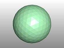 Subdivision with 25*20 faces |
A different second option is to construct new edges by splitting the angle γ1 into regular pieces γs=γ1/s, and to rotate in steps by along the great circle until it reaches . The rotation matrix could be computed by first constructing the axis of the rotation via the cross product and normalizing it. The rotation matrix is for example computed with Mercer's theorem by using this rotation axis with eigenvalue 1 and the two orthogonal axes with complex eigenvalues , .


History
The earliest use of the (icosahedral) geodesic grid in geophysical modeling dates back to 1968 and the work by Sadourny, Arakawa, and Mintz[7] and Williamson.[8] [9] Later work expanded on this base.[10][11][12][13][14]
A generalization to any number of dimensions, spherical design, was developed in 1984.
References
- ↑ White, D; Kimerling AJ; Overton WS (1992). "Cartographic and geometric components of a global sampling design for environmental monitoring.". Cartography and Geographic Information Systems. 19 (1): 5–22. doi:10.1559/152304092783786636.
- ↑ Clarke, Keith C (2000). "Criteria and Measures for the Comparison of Global Geocoding Systems". Discrete Global Grids: Goodchild, M. F. and A. J. Kimerling, Eds.
- ↑ Mahdavi-Amiri, Ali; Harrison.E; Samavati.F (2014). "hexagonal connectivity maps for digital earth". International Journal of Digital Earth. Bibcode:2015IJDE....8..750M. doi:10.1080/17538947.2014.927597.
- ↑ Mahdavi-Amiri, Ali; Bhojani.F; Samavati.F (2013). "One-to-two digital earth". Lecture Notes on Computational Sciences. doi:10.1007/978-3-642-41939-3_67.
- ↑ Silla, Estanislao (1991). "GEPOL: an improved description of molecular surface. II. Computing the molecular area and volume". J. Comp. Chem. 12. doi:10.1002/jcc.540120905.
- ↑ Fekete, György (1990). "Rendering and managing spherical data with sphere quadtrees".
- ↑ Sadourny, R.; A. Arakawa; Y. Mintz (1968). "Integration of the non-divergent barotropic vorticity equation with an icosahedral-hexagonal grid for the sphere". Monthly weather review. 96 (6): 351–356. Bibcode:1968MWRv...96..351S. doi:10.1175/1520-0493(1968)096<0351:IOTNBV>2.0.CO;2.
- ↑ Williamson, D. L. (1968). "Integration of the barotropic vorticity equation on a spherical geodesic grid". Tellus. 20 (4): 642–653. doi:10.1111/j.2153-3490.1968.tb00406.x.
- ↑ Williamson, 1969
- ↑ Cullen, M. J. P. (1974). "Integrations of the primitive equations on a sphere using the finite-element method". Quarterly Journal of the Royal Meteorological Society. 100 (426): 555–562. Bibcode:1974QJRMS.100..555C. doi:10.1002/qj.49710042605.
- ↑ Cullen and Hall, 1979.
- ↑ Masuda, Y. Girard1 (1987). "An integration scheme of the primitive equation model with an icosahedral-hexagonal grid system and its application to the shallow-water equations". Short- and Medium-Range Numerical Weather Prediction. Japan Meteorological Society. pp. 317–326.
- ↑ Heikes, Ross; David A. Randall (1995). "Numerical integration of the shallow-water equations on a twisted icosahedral grid. Part I: Basic design and results of tests". Monthly Weather Review. 123 (6): 1862–1880. Bibcode:1995MWRv..123.1862H. doi:10.1175/1520-0493(1995)123<1862:NIOTSW>2.0.CO;2.Heikes, Ross; David A. Randall (1995). "Numerical integration of the shallow-water equations on a twisted icosahedral grid. Part II: A detailed description of the grid and an analysis of numerical accuracy". Monthly Weather Review. 123 (6): 1881–1887. Bibcode:1995MWRv..123.1881H. doi:10.1175/1520-0493(1995)123<1881:NIOTSW>2.0.CO;2.
- ↑ Randall et al., 2000; Randall et al., 2002.
External links
- BUGS climate model page on geodesic grids
- Discrete Global Grids page at the Computer Science department at Southern Oregon University
- the PYXIS innovation Digital Earth Reference Model .
- Interpolation on spherical geodesic grids: A comparative study