Flamant solution

The Flamant solution provides expressions for the stresses and displacements in a linear elastic wedge loaded by point forces at its sharp end. This solution was developed by A. Flamant [1] in 1892 by modifying the three-dimensional solution of Boussinesq.
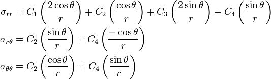
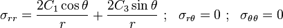
The stresses predicted by the Flamant solution are (in polar coordinates)

where  are constants that are determined from the boundary conditions and the geometry of the wedge (i.e., the angles
  ) and satisfy
where  are the applied forces.
The wedge problem is self-similar and has no inherent length scale. Also, all quantities can be expressed in the separated-variable form  . The stresses vary as
  .
.
Forces acting on a half-plane
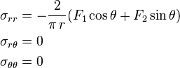
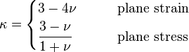
For the special case where  ,
,  , the wedge is converted into a half-plane with a normal force and a tangential force. In that case
Therefore the stresses are
and the displacements are (using Michell's solution)
![\begin{align}
u_r & = -\cfrac{1}{4\pi\mu}\left[F_1\{(\kappa-1)\theta\sin\theta - \cos\theta + (\kappa+1)\ln r\cos\theta\} + \right. \\
& \qquad \qquad \left. F_2\{(\kappa-1)\theta\cos\theta + \sin\theta - (\kappa+1)\ln r\sin\theta\}\right]\\
u_\theta & = -\cfrac{1}{4\pi\mu}\left[F_1\{(\kappa-1)\theta\cos\theta - \sin\theta - (\kappa+1)\ln r\sin\theta\} - \right. \\
& \qquad \qquad \left. F_2\{(\kappa-1)\theta\sin\theta + \cos\theta + (\kappa+1)\ln r\cos\theta\}\right]
\end{align}](../I/m/496b6f7767598c7f1ed4d634ef2210bb.png)
The  dependence of the displacements implies that the displacement grows the further one moves from the point of application of the force (and is unbounded at infinity). This feature of the Flamant solution is confusing and appears unphysical. For a discussion of the issue see http://imechanica.org/node/319.
Displacements at the surface of the half-plane
The displacements in the  directions at the surface of the half-plane are given by
where
 is the Poisson's ratio,
  is the shear modulus, and
Derivation of Flamant solution
If we assume the stresses to vary as , we can pick terms containing  in the stresses from Michell's solution. Then the Airy stress function can be expressed as

Therefore, from the tables in Michell's solution, we have
The constants  can then, in principle, be determined from the wedge geometry and the applied boundary conditions.
However, the concentrated loads at the vertex are difficult to express in terms of traction boundary conditions because
- the unit outward normal at the vertex is undefined
- the forces are applied at a point (which has zero area) and hence the traction at that point is infinite.

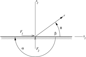
To get around this problem, we consider a bounded region of the wedge and consider equilibrium of the bounded wedge.[2][3] Let the bounded wedge have two traction free surfaces and a third surface in the form of an arc of a circle with radius  . Along the arc of the circle, the unit outward normal is
  where the basis vectors are
  . The tractions on the arc are

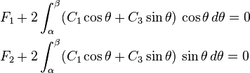
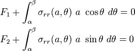
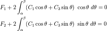
Next, we examine the force and moment equilibrium in the bounded wedge and get
![\begin{align}
\sum f_1 & = F_1 + \int_{\alpha}^{\beta} \left[\sigma_{rr}(a,\theta)~\cos\theta
- \sigma_{r\theta}(a,\theta)~\sin\theta\right]~a~d\theta = 0 \\
\sum f_2 & = F_2 + \int_{\alpha}^{\beta} \left[\sigma_{rr}(a,\theta)~\sin\theta
+ \sigma_{r\theta}(a,\theta)~\cos\theta\right]~a~d\theta = 0 \\
\sum m_3 & = \int_{\alpha}^{\beta} \left[a~\sigma_{r\theta}(a,\theta)\right]~a~d\theta = 0
\end{align}](../I/m/c67b1d45e05b5ad20a385660875e6915.png)
We require that these equations be satisfied for all values of and thereby satisfy the boundary conditions.
The traction-free boundary conditions on the edges  and
and  also imply that

except at the point  .
.
If we assume that  everywhere, then the traction-free conditions and the moment equilibrium equation are satisfied and we are left with
and  along
along 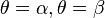 except at the point . But the field everywhere also satisfies the force equilibrium equations. Hence this must be the solution. Also, the assumption implies that
 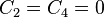 .
.
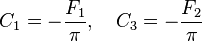
Therefore,
To find a particular solution for  we have to plug in the expression for into the force equilibrium equations to get a system of two equations which have to be solved for :
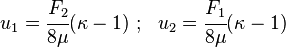
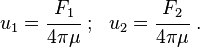
Forces acting on a half-plane
If we take and , the problem is converted into one where a normal force  and a tangential force
  act on a half-plane. In that case, the force equilibrium equations take the form
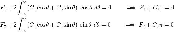
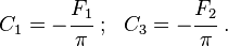
Therefore
The stresses for this situation are

Using the displacement tables from the Michell solution, the displacements for this case are given by
Displacements at the surface of the half-plane
To find expressions for the displacements at the surface of the half plane, we first find the displacements for positive  (
( ) and negative (
 ) keeping in mind that
  along these locations.
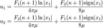
For we have
![\begin{align}
u_r = u_1 & = \cfrac{F_1}{4\pi\mu}\left[1 - (\kappa+1)\ln |x_1|\right] \\
u_\theta = u_2 & = \cfrac{F_2}{4\pi\mu}\left[1 + (\kappa+1)\ln |x_1|\right]
\end{align}](../I/m/012f3ed1e4be64f79a12b95ce9feeb39.png)
For we have
![\begin{align}
u_r = -u_1 & = -\cfrac{F_1}{4\pi\mu}\left[1 - (\kappa+1)\ln |x_1|\right] +
\cfrac{F_2}{4\mu}(\kappa-1)\\
u_\theta = -u_2 & = \cfrac{F_1}{4\mu}(\kappa-1) -
\cfrac{F_2}{4\pi\mu}\left[1 + (\kappa+1)\ln |x_1|\right]
\end{align}](../I/m/26a4cf9df1eab90c84bdc76e8401d09b.png)
We can make the displacements symmetric around the point of application of the force by adding rigid body displacements (which does not affect the stresses)
and removing the redundant rigid body displacements
Then the displacements at the surface can be combined and take the form
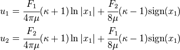
where
References
- ↑ A. Flamant. (1892). Sur la répartition des pressions dans un solide rectangulaire chargé transversalement. Compte. Rendu. Acad. Sci. Paris, vol. 114, p. 1465.
- ↑ Slaughter, W. S. (2002). The Linearized Theory of Elasticity. Birkhauser, Boston, p. 294.
- ↑ J. R. Barber, 2002, Elasticity: 2nd Edition, Kluwer Academic Publishers.