Elliptic boundary value problem

Shows a region where a differential equation is valid and the associated boundary values

In mathematics, an elliptic boundary value problem is a special kind of boundary value problem which can be thought of as the stable state of an evolution problem. For example, the Dirichlet problem for the Laplacian gives the eventual distribution of heat in a room several hours after the heating is turned on.

Differential equations describe a large class of natural phenomena, from the heat equation describing the evolution of heat in (for instance) a metal plate, to the Navier-Stokes equation describing the movement of fluids, including Einstein's equations describing the physical universe in a relativistic way. Although all these equations are boundary value problems, they are further subdivided into categories. This is necessary because each category must be analyzed using different techniques. The present article deals with the category of boundary value problems known as linear elliptic problems.

Boundary value problems and partial differential equations specify relations between two or more quantities. For instance, in the heat equation, the rate of change of temperature at a point is related to the difference of temperature between that point and the nearby points so that, over time, the heat flows from hotter points to cooler points. Boundary value problems can involve space, time and other quantities such as temperature, velocity, pressure, magnetic field, etc...

Some problems do not involve time. For instance, if one hangs a clothesline between the house and a tree, then in the absence of wind, the clothesline will not move and will adopt a gentle hanging curved shape known as the catenary.^[1] This curved shape can be computed as the solution of a differential equation relating position, tension, angle and gravity, but since the shape does not change over time, there is no time variable.

Elliptic boundary value problems are a class of problems which do not involve the time variable, and instead only depend on space variables.

It is not possible to discuss elliptic boundary value problems in more detail without referring to calculus in multiple variables.

Unless otherwise noted, all facts presented in this article can be found in.^[2]

The main example

In two dimensions, let $x,y$ be the coordinates. We will use the notation $u_x, u_{xx}$ for the first and second partial derivatives of $u$ with respect to $x$ , and a similar notation for $y$ . We will use the symbols $D_x$ and $D_y$ for the partial differential operators in $x$ and $y$ . The second partial derivatives will be denoted $D_x^2$ and $D_y^2$ . We also define the gradient 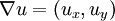$\nabla u = (u_x,u_y)$ , the Laplace operator 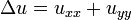$\Delta u = u_{xx}+u_{yy}$ and the divergence 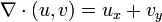$\nabla \cdot (u,v) = u_x + v_y$ . Note from the definitions that $\Delta u = \nabla \cdot (\nabla u)$ .

The main example for boundary value problems is the Laplace operator,

\Delta u = f \text{ in }\Omega,

u = 0 \text { on }\partial \Omega;

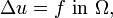
where $\Omega$ is a region in the plane and $\partial \Omega$ is the boundary of that region. The function $f$ is known data and the solution $u$ is what must be computed. This example has the same essential properties as all other elliptic boundary value problems.

The solution $u$ can be interpreted as the stationary or limit distribution of heat in a metal plate shaped like $\Omega$ , if this metal plate has its boundary adjacent to ice (which is kept at zero degrees, thus the Dirichlet boundary condition.) The function $f$ represents the intensity of heat generation at each point in the plate (perhaps there is an electric heater resting on the metal plate, pumping heat into the plate at rate $f(x)$ , which does not vary over time, but may be nonuniform in space on the metal plate.) After waiting for a long time, the temperature distribution in the metal plate will approach $u$ .

Nomenclature

Let $Lu=a u_{xx} + b u_{yy}$ where $a$ and $b$ are constants. $L=aD_x^2+bD_y^2$ is called a second order differential operator. If we formally replace the derivatives $D_x$ by $x$ and $D_y$ by $y$ , we obtain the expression

a x^2 + b y^2

If we set this expression equal to some constant $k$ , then we obtain either an ellipse (if $a,b,k$ are all the same sign) or a hyperbola (if $a$ and $b$ are of opposite signs.) For that reason, $L$ is said to be elliptic when $ab>0$ and hyperbolic if $ab<0$ . Similarly, the operator $L=D_x+D_y^2$ leads to a parabola, and so this $L$ is said to be parabolic.

We now generalize the notion of ellipticity. While it may not be obvious that our generalization is the right one, it turns out that it does preserve most of the necessary properties for the purpose of analysis.

General linear elliptic boundary value problems of the second degree

Let $x_1,...,x_n$ be the space variables. Let $a_{ij}(x), b_i(x), c(x)$ be real valued functions of $x=(x_1,...,x_n)$ . Let $L$ be a second degree linear operator. That is,

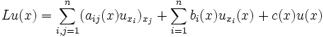Lu(x)=\sum_{i,j=1}^n (a_{ij} (x) u_{x_i})_{x_j} + \sum_{i=1}^n b_i(x) u_{x_i}(x) + c(x) u(x)

(divergence form).

Lu(x)=\sum_{i,j=1}^n a_{ij} (x) u_{x_i x_j} + \sum_{i=1}^n \tilde b_i u_{x_i}(x) + c(x) u(x)

(nondivergence form)

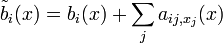
We have used the subscript $\cdot_{x_i}$ to denote the partial derivative with respect to the space variable $x_i$ . The two formulae are equivalent, provided that

\tilde b_i(x) = b_i(x) + \sum_j a_{ij,x_j}(x)

In matrix notation, we can let $a(x)$ be an $n \times n$ matrix valued function of $x$ and $b(x)$ be a $n$ -dimensional column vector-valued function of $x$ , and then we may write

Lu = \nabla \cdot (a \nabla u) + b^T \nabla u + c u

(divergence form).

One may assume, without loss of generality, that the matrix $a$ is symmetric (that is, for all 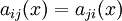$i,j,x$ , $a_{ij}(x)=a_{ji}(x)$ . We make that assumption in the rest of this article.

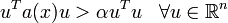
We say that the operator $L$ is elliptic if, for some constant $\alpha>0$ , any of the following equivalent conditions hold:

$\lambda_{\min} (a(x)) > \alpha \;\;\; \forall x$ (see eigenvalue).
$u^T a(x) u > \alpha u^T u \;\;\; \forall u \in \mathbb{R}^n$ .
$\sum_{i,j=1}^n a_{ij} u_i u_j > \alpha \sum_{i=1}^n u_i^2 \;\;\; \forall u \in \mathbb{R}^n$ .

An elliptic boundary value problem is then a system of equations like

Lu=f \text{ in } \Omega

(the PDE) and

u=0 \text{ on } \partial \Omega

(the boundary value).

This particular example is the Dirichlet problem. The Neumann problem is

Lu=f \text{ in } \Omega

and

u_\nu = g \text{ on } \partial \Omega

where $u_\nu$ is the derivative of $u$ in the direction of the outwards pointing normal of $\partial \Omega$ . In general, if $B$ is any trace operator, one can construct the boundary value problem

Lu=f \text{ in } \Omega

and

Bu=g \text{ on } \partial \Omega

In the rest of this article, we assume that $L$ is elliptic and that the boundary condition is the Dirichlet condition $u=0 \text{ on }\partial \Omega$ .

Sobolev spaces

The analysis of elliptic boundary value problems requires some fairly sophisticated tools of functional analysis. We require the space $H^1(\Omega)$ , the Sobolev space of "once-differentiable" functions on $\Omega$ , such that both the function $u$ and its partial derivatives $u_{x_i}$ , $i=1,\dots,n$ are all square integrable. There is a subtlety here in that the partial derivatives must be defined "in the weak sense" (see the article on Sobolev spaces for details.) The space $H^1$ is a Hilbert space, which accounts for much of the ease with which these problems are analyzed.

The discussion in details of Sobolev spaces is beyond the scope of this article, but we will quote required results as they arise.

Unless otherwise noted, all derivatives in this article are to be interpreted in the weak, Sobolev sense. We use the term "strong derivative" to refer to the classical derivative of calculus. We also specify that the spaces $C^k$ , $k=0,1,\dots$ consist of functions that are $k$ times strongly differentiable, and that the $k$ th derivative is continuous.

Weak or variational formulation

The first step to cast the boundary value problem as in the language of Sobolev spaces is to rephrase it in its weak form. Consider the Laplace problem $\Delta u = f$ . Multiply each side of the equation by a "test function" $\varphi$ and integrate by parts using Green's theorem to obtain

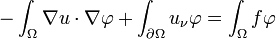-\int_\Omega \nabla u \cdot \nabla \varphi + \int_{\partial \Omega} u_\nu \varphi = \int_\Omega f \varphi

We will be solving the Dirichlet problem, so that $u=0\text{ on }\partial \Omega$ . For technical reasons, it is useful to assume that $\varphi$ is taken from the same space of functions as $u$ is so we also assume that $\varphi=0\text{ on }\partial \Omega$ . This gets rid of the $\int_{\partial \Omega}$ term, yielding

A(u,\varphi) = F(\varphi)

(*)

where

A(u,\varphi) = \int_\Omega \nabla u \cdot \nabla \varphi

and

F(\varphi) = -\int_\Omega f \varphi

If $L$ is a general elliptic operator, the same reasoning leads to the bilinear form

A(u,\varphi) = \int_\Omega \nabla u ^T a \nabla \varphi - \int_\Omega b^T \nabla u \varphi - \int_\Omega c u \varphi

We do not discuss the Neumann problem but note that it is analyzed in a similar way.

Continuous and coercive bilinear forms

The map $A(u,\varphi)$ is defined on the Sobolev space $H^1_0\subset H^1$ of functions which are once differentiable and zero on the boundary $\partial \Omega$ , provided we impose some conditions on $a,b,c$ and $\Omega$ . There are many possible choices, but for the purpose of this article, we will assume that

$a_{ij}(x)$ is continuously differentiable on $\bar\Omega$ for $i,j=1,\dots,n,$
$b_i(x)$ is continuous on $\bar\Omega$ for $i=1,\dots,n,$
$c(x)$ is continuous on $\bar\Omega$ and
$\Omega$ is bounded.

The reader may verify that the map $A(u,\varphi)$ is furthermore bilinear and continuous, and that the map $F(\varphi)$ is linear in $\varphi$ , and continuous if (for instance) $f$ is square integrable.

We say that the map $A$ is coercive if there is an $\alpha>0$ for all $u,\varphi \in H_0^1(\Omega)$ ,

A(u,\varphi) \geq \alpha \int_\Omega \nabla u \cdot \nabla \varphi.

This is trivially true for the Laplacian (with $\alpha=1$ ) and is also true for an elliptic operator if we assume $b = 0$ and $c \leq 0$ . (Recall that $u^T a u > \alpha u^T u$ when $L$ is elliptic.)

Existence and uniqueness of the weak solution

One may show, via the Lax–Milgram lemma, that whenever $A(u,\varphi)$ is coercive and $F(\varphi)$ is continuous, then there exists a unique solution $u\in H_0^1(\Omega)$ to the weak problem (*).

If further $A(u,\varphi)$ is symmetric (i.e., $b=0$ ), one can show the same result using the Riesz representation theorem instead.

This relies on the fact that $A(u,\varphi)$ forms an inner product on $H_0^1(\Omega)$ , which itself depends on Poincaré's inequality.

Strong solutions

We have shown that there is a $u\in H_0^1(\Omega)$ which solves the weak system, but we do not know if this $u$ solves the strong system

Lu=f\text{ in }\Omega,

u=0\text{ on }\partial \Omega,

Even more vexing is that we are not even sure that $u$ is twice differentiable, rendering the expressions $u_{x_i x_j}$ in $Lu$ apparently meaningless. There are many ways to remedy the situation, the main one being regularity.

Regularity

A regularity theorem for a linear elliptic boundary value problem of the second order takes the form

Theorem If (some condition), then the solution $u$ is in $H^2(\Omega)$ , the space of "twice differentiable" functions whose second derivatives are square integrable.

There is no known simple condition necessary and sufficient for the conclusion of the theorem to hold, but the following conditions are known to be sufficient:

The boundary of $\Omega$ is $C^2$ , or
$\Omega$ is convex.

It may be tempting to infer that if $\partial \Omega$ is piecewise $C^2$ then $u$ is indeed in $H^2$ , but that is unfortunately false.

Almost everywhere solutions

In the case that $u \in H^2(\Omega)$ then the second derivatives of $u$ are defined almost everywhere, and in that case $Lu=f$ almost everywhere.

Strong solutions

One may further prove that if the boundary of $\Omega \subset \mathbb{R}^n$ is a smooth manifold and $f$ is infinitely differentiable in the strong sense, then $u$ is also infinitely differentiable in the strong sense. In this case, $Lu=f$ with the strong definition of the derivative.

The proof of this relies upon an improved regularity theorem that says that if $\partial \Omega$ is $C^k$ and $f \in H^{k-2}(\Omega)$ , $k\geq 2$ , then $u\in H^k(\Omega)$ , together with a Sobolev imbedding theorem saying that functions in $H^k(\Omega)$ are also in $C^m(\bar \Omega)$ whenever $0 \leq m < k-n/2$ .

Numerical solutions

While in exceptional circumstances, it is possible to solve elliptic problems explicitly, in general it is an impossible task. The natural solution is to approximate the elliptic problem with a simpler one and to solve this simpler problem on a computer.

Because of the good properties we have enumerated (as well as many we have not), there are extremely efficient numerical solvers for linear elliptic boundary value problems (see finite element method, finite difference method and spectral method for examples.)

Eigenvalues and eigensolutions

Another Sobolev imbedding theorem states that the inclusion $H^1\subset L^2$ is a compact linear map. Equipped with the spectral theorem for compact linear operators, one obtains the following result.

Theorem Assume that $A(u,\varphi)$ is coercive, continuous and symmetric. The map $S : f \rightarrow u$ from $L^2(\Omega)$ to $L^2(\Omega)$ is a compact linear map. It has a basis of eigenvectors $u_1, u_2, \dots \in H^1(\Omega)$ and matching eigenvalues $\lambda_1,\lambda_2,\dots \in \mathbb{R}$ such that

$Su_k = \lambda_k u_k, k=1,2,\dots,$
$\lambda_k \rightarrow 0$ as $k \rightarrow \infty$ ,
$\lambda_k \gneqq 0\;\;\forall k$ ,
$\int_\Omega u_j u_k = 0$ whenever $j \neq k$ and
$\int_\Omega u_j u_j = 1$ for all $j=1,2,\dots\,.$

Series solutions and the importance of eigensolutions

If one has computed the eigenvalues and eigenvectors, then one may find the "explicit" solution of $Lu=f$ ,

u=\sum_{k=1}^\infty \hat u(k) u_k

via the formula

\hat u(k) = \lambda_k \hat f(k) ,\;\;k=1,2,\dots

where

\hat f(k) = \int_{\Omega} f(x) u_k(x) \, dx.

(See Fourier series.)

The series converges in $L^2$ . Implemented on a computer using numerical approximations, this is known as the spectral method.

An example

Consider the problem

u-u_{xx}-u_{yy}=f(x,y)=xy

(0,1)\times(0,1),

u(x,0)=u(x,1)=u(0,y)=u(1,y)=0 \;\;\forall (x,y)\in(0,1)\times(0,1)

(Dirichlet conditions).

The reader may verify that the eigenvectors are exactly

u_{jk}(x,y)=\sin(\pi jx)\sin(\pi ky)

j,k\in \mathbb{N}

with eigenvalues

\lambda_{jk}={ 1 \over 1+\pi^2 j^2+\pi^2 k^2 }.

The Fourier coefficients of $g(x)=x$ can be looked up in a table, getting $\hat g(n) = { (-1)^{n+1} \over \pi n }$ . Therefore,

\hat f(j,k) = { (-1)^{j+k+1} \over \pi^2 jk }

yielding the solution

u(x,y) = \sum_{j,k=1}^\infty { (-1)^{j+k+1} \over \pi^2 jk (1+\pi^2 j^2+\pi^2 k^2) } \sin(\pi jx) \sin (\pi ky).

Maximum principle

There are many variants of the maximum principle. We give a simple one.

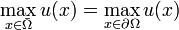Theorem. (Weak maximum principle.) Let $u \in C^2(\Omega) \cap C^1(\bar \Omega)$ , and assume that $c(x)=0\;\forall x\in\Omega$ . Say that $Lu \leq 0$ in $\Omega$ . Then $\max_{x \in \bar \Omega} u(x) = \max_{x \in \partial \Omega} u(x)$ . In other words, the maximum is attained on the boundary.

A strong maximum principle would conclude that 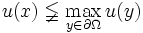$u(x) \lneqq \max_{y \in \partial \Omega} u(y)$ for all $x \in \Omega$ unless $u$ is constant.

References

↑ Swetz, Faauvel, Bekken, "Learn from the Masters", 1997, MAA ISBN 0-88385-703-0, pp.128-9
↑ Partial Differential Equations by Lawrence C. Evans. American Mathematical Society, Providence, RI, 1998. Graduate Studies in Mathematics 19.

This article is issued from Wikipedia - version of the 12/28/2015. The text is available under the Creative Commons Attribution/Share Alike but additional terms may apply for the media files.