Dirac equation in the algebra of physical space

Algebra of physical space (APS)

Mathematical concepts	Paravector algebra

Applications in physics	Special relativity with APS Dirac equation with APS

The Dirac equation, as the relativistic equation that describes spin 1/2 particles in quantum mechanics can be written in terms of the Algebra of physical space (APS), which is a case of a Clifford algebra or geometric algebra that is based in the use of paravectors.

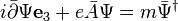
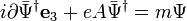
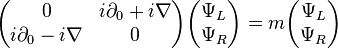
The Dirac equation in APS, including the electromagnetic interaction, reads

i \bar{\partial} \Psi\mathbf{e}_3 + e \bar{A} \Psi = m \bar{\Psi}^\dagger

Another form of the Dirac equation in terms of the Space time algebra was given earlier by David Hestenes.

In general, the Dirac equation in the formalism of geometric algebra has the advantage of providing a direct geometric interpretation.

Relation with the standard form

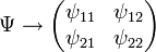
The spinor can be written in a null basis as

\Psi = \psi_{11} P_3 - \psi_{12} P_3 \mathbf{e}_1 + \psi_{21} \mathbf{e}_1 P_3 + \psi_{22} \bar{P}_3,

such that the representation of the spinor in terms of the Pauli matrices is

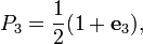
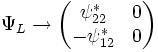
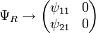
\Psi \rightarrow \begin{pmatrix} \psi_{11} & \psi_{12} \\ \psi_{21} & \psi_{22} \end{pmatrix}

\bar{\Psi}^\dagger \rightarrow \begin{pmatrix} \psi_{22}^* & -\psi_{21}^* \\ -\psi_{12}^* & \psi_{11}^* \end{pmatrix}

The standard form of the Dirac equation can be recovered by decomposing the spinor in its right and left-handed spinor components, which are extracted with the help of the projector

P_3 = \frac{1}{2}( 1 + \mathbf{e}_3),

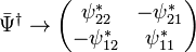
such that

\Psi_L = \bar{\Psi}^\dagger P_3

\Psi_R = \Psi P_3^{ }

with the following matrix representation

\Psi_L \rightarrow \begin{pmatrix} \psi_{22}^* & 0 \\ -\psi_{12}^* & 0 \end{pmatrix}

\Psi_R \rightarrow \begin{pmatrix} \psi_{11} & 0 \\ \psi_{21} & 0 \end{pmatrix}

The Dirac equation can be also written as

i \partial \bar{\Psi}^\dagger \mathbf{e}_3 + e A \bar{\Psi}^\dagger = m \Psi

Without electromagnetic interaction, the following equation is obtained from the two equivalent forms of the Dirac equation

\begin{pmatrix} 0 & i \bar{\partial}\\ i \partial & 0 \end{pmatrix} \begin{pmatrix} \bar{\Psi}^\dagger P_3 \\ \Psi P_3 \end{pmatrix} = m \begin{pmatrix} \bar{\Psi}^\dagger P_3 \\ \Psi P_3 \end{pmatrix}

so that

\begin{pmatrix} 0 & i \partial_0 + i\nabla \\ i \partial_0 - i \nabla & 0 \end{pmatrix} \begin{pmatrix} \Psi_L \\ \Psi_R \end{pmatrix} = m \begin{pmatrix} \Psi_L \\ \Psi_R \end{pmatrix}

or in matrix representation

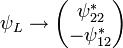
i \left( \begin{pmatrix} 0 & 1 \\ 1 & 0 \end{pmatrix} \partial_0 + \begin{pmatrix} 0 & \sigma \\ -\sigma & 0 \end{pmatrix} \cdot \nabla \right) \begin{pmatrix} \psi_L \\ \psi_R \end{pmatrix} = m \begin{pmatrix} \psi_L \\ \psi_R \end{pmatrix},

where the second column of the right and left spinors can be dropped by defining the single column chiral spinors as

\psi_L \rightarrow \begin{pmatrix} \psi_{22}^* \\ -\psi_{12}^* \end{pmatrix}

\psi_R \rightarrow \begin{pmatrix} \psi_{11} \\ \psi_{21} \end{pmatrix}

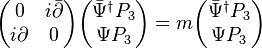
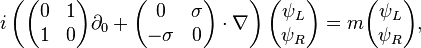
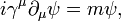
The standard relativistic covariant form of the Dirac equation in the Weyl representation can be easily identified $i \gamma^{\mu} \partial_{\mu} \psi = m \psi,$ such that

\psi_= \begin{pmatrix} \psi_{22}^* \\ -\psi_{12}^* \\ \psi_{11} \\ \psi_{21} \end{pmatrix}

Given two spinors $\Psi$ and $\Phi$ in APS and their respective spinors in the standard form as $\psi$ and $\phi$ , one can verify the following identity

\phi^\dagger \gamma^0 \psi = \langle \bar{\Phi}\Psi + (\bar{\Psi}\Phi)^\dagger \rangle_S

such that

\psi^\dagger \gamma^0 \psi = 2 \langle \bar{\Psi}\Psi \rangle_{S R}

Electromagnetic gauge

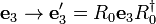
The Dirac equation is invariant under a global right rotation applied on the spinor of the type

\Psi \rightarrow \Psi^\prime = \Psi R_0

so that the kinetic term of the Dirac equation transforms as

i\bar{\partial} \Psi \mathbf{e}_3 \rightarrow i\bar{\partial} \Psi R_0 \mathbf{e}_3 R_0^\dagger R_0 = ( i\bar{\partial} \Psi \mathbf{e}_3^\prime ) R_0,

where we identify the following rotation

\mathbf{e}_3 \rightarrow \mathbf{e}_3^\prime = R_0 \mathbf{e}_3 R_0^\dagger

The mass term transforms as

m \overline{\Psi^\dagger} \rightarrow m \overline{(\Psi R_0)^\dagger} = m \overline{ \Psi^\dagger }R_0,

so that we can verify the invariance of the form of the Dirac equation. A more demanding requirement is that the Dirac equation should be invariant under a local gauge transformation of the type 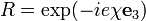$R=\exp(-i e \chi \mathbf{e}_3)$

In this case, the kinetic term transforms as

i\bar{\partial} \Psi \mathbf{e}_3 \rightarrow (i \bar{\partial} \Psi) R \mathbf{e}_3 + (e\bar{\partial}\chi) \Psi R

so that the left side of the Dirac equation transforms covariantly as

i\bar{\partial} \Psi \mathbf{e}_3 -e \bar{A}\Psi \rightarrow (i\bar{\partial} \Psi R \mathbf{e}_3 R^\dagger -e \overline{(A + \partial \chi)}\Psi)R,

where we identify the need to perform an electromagnetic gauge transformation. The mass term transforms as in the case with global rotation, so, the form of the Dirac equation remains invariant.

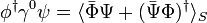
Current

The current is defined as

J = \Psi\Psi^\dagger,

which satisfies the continuity equation

\left\langle \bar{\partial} J \right\rangle_{S}=0

Second order Dirac equation

An application of the Dirac equation on itself leads to the second order Dirac equation

(-\partial \bar{\partial} + A \bar{A}) \Psi - i( 2e\left\langle A \bar{\partial} \right\rangle_S + eF) \Psi \mathbf{e}_3 = m^2 \Psi

Free particle solutions

Positive energy solutions

A solution for the free particle with momentum $p = p^0 + \mathbf{p}$ and positive energy $p^0>0$ is

\Psi = \sqrt{\frac{p}{m}} R(0) \exp(-i\left\langle p \bar{x}\right\rangle_S \mathbf{e}_3).

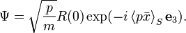
This solution is unimodular

\Psi \bar{\Psi} = 1

and the current resembles the classical proper velocity

u = \frac{p}{m}

J = \Psi {\Psi}^\dagger = \frac{p}{m}

Negative energy solutions

A solution for the free particle with negative energy and momentum $p = -|p^0| - \mathbf{p} = - p^\prime$ is

\Psi = i\sqrt{\frac{p^\prime}{m}} R(0) \exp(i\left\langle p^\prime \bar{x}\right\rangle_S \mathbf{e}_3) ,

This solution is anti-unimodular

\Psi \bar{\Psi} = -1

and the current resembles the classical proper velocity $u = \frac{p}{m}$

J = \Psi {\Psi}^\dagger = -\frac{p}{m},

but with a remarkable feature: "the time runs backwards"

\frac{d t}{d \tau} = \left\langle \frac{p}{m} \right\rangle_S < 0

Dirac Lagrangian

The Dirac Lagrangian is

L = \langle i \partial \bar{\Psi}^\dagger \mathbf{e}_3 \bar{\Psi} - e A \bar{\Psi}^\dagger \bar{\Psi} -m \Psi \bar{\Psi} \rangle_S

References

Textbooks

Baylis, William (2002). Electrodynamics: A Modern Geometric Approach (2nd ed.). Birkhäuser. ISBN 0-8176-4025-8
W. E. Baylis, editor, Clifford (Geometric) Algebra with Applications to Physics, Mathematics, and Engineering, Birkhäuser, Boston 1996.

Articles

Baylis, William, Classical eigenspinors and the Dirac equation, Phys. Rev. A 45, 4293–4302 (1992)
Hestenes D., Observables, operators, and complex numbers in the Dirac theory, J. Math. Phys. 16, 556 (1975)

This article is issued from Wikipedia - version of the 3/18/2016. The text is available under the Creative Commons Attribution/Share Alike but additional terms may apply for the media files.