Describing function
In control systems theory, the describing function (DF) method, developed by Nikolay Mitrofanovich Krylov and Nikolay Bogoliubov in the 1930s,[1][2] and extended by Ralph Kochenburger[3] is an approximate procedure for analyzing certain nonlinear control problems. It is based on quasi-linearization, which is the approximation of the non-linear system under investigation by a linear time-invariant (LTI) transfer function that depends on the amplitude of the input waveform. By definition, a transfer function of a true LTI system cannot depend on the amplitude of the input function because an LTI system is linear. Thus, this dependence on amplitude generates a family of linear systems that are combined in an attempt to capture salient features of the non-linear system behavior. The describing function is one of the few widely applicable methods for designing nonlinear systems, and is very widely used as a standard mathematical tool for analyzing limit cycles in closed-loop controllers, such as industrial process controls, servomechanisms, and electronic oscillators.
The method
Consider feedback around a discontinuous (but piecewise continuous) nonlinearity (e.g., an amplifier with saturation, or an element with deadband effects) cascaded with a slow stable linear system. Depending on the amplitude of the output of the linear system, the feedback presented to the nonlinearity will be in a different continuous region. As the output of the linear system decays, the nonlinearity may move into a different continuous region. This switching from one continuous region to another can generate periodic oscillations. The describing function method attempts to predict characteristics of those oscillations (e.g., their fundamental frequency) by assuming that the slow system acts like a low-pass or bandpass filter that concentrates all energy around a single frequency. Even if the output waveform has several modes, the method can still provide intuition about properties like frequency and possibly amplitude; in this case, the describing function method can be thought of as describing the sliding mode of the feedback system.
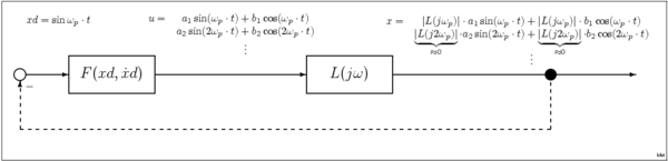
Using this low-pass assumption, the system response can be described by one of a family of sinusoidal waveforms; in this case the system would be characterized by a sine input describing function (SIDF) giving the system response to an input consisting of a sine wave of amplitude A and frequency . This SIDF is a modification of the transfer function used to characterize linear systems. In a quasi-linear system, when the input is a sine wave, the output will be a sine wave of the same frequency but with a scaled amplitude and shifted phase as given by . Many systems are approximately quasi-linear in the sense that although the response to a sine wave is not a pure sine wave, most of the energy in the output is indeed at the same frequency as the input. This is because such systems may possess intrinsic low-pass or bandpass characteristics such that harmonics are naturally attenuated, or because external filters are added for this purpose. An important application of the SIDF technique is to estimate the oscillation amplitude in sinusoidal electronic oscillators.


Other types of describing functions that have been used are DFs for level inputs and for Gaussian noise inputs. Although not a complete description of the system, the DFs often suffice to answer specific questions about control and stability. DF methods are best for analyzing systems with relatively weak nonlinearities. In addition the higher order sinusoidal input describing functions (HOSIDF), describe the response of a class of nonlinear systems at harmonics of the input frequency of a sinusoidal input. The HOSIDFs are an extension of the SIDF for systems where the nonlinearities are significant in the response.
Caveats
Although the describing function method can produce reasonably accurate results for a wide class of systems, it can fail badly for others. For example, the method can fail if the system emphasizes higher harmonics of the nonlinearity. Such examples have been presented by Tzypkin for bang–bang systems.[4] A fairly similar example is a closed-loop oscillator consisting of a non-inverting Schmitt trigger followed by an inverting integrator that feeds back its output to the Schmitt trigger's input. The output of the Schmitt trigger is going to be a square waveform, while that of the integrator (following it) is going to have a triangle waveform with peaks coinciding with the transitions in the square wave. Each of these two oscillator stages lags the signal exactly by 90 degrees (relative to its input). If one were to perform DF analysis on this circuit, the triangle wave at the Schmitt trigger's input would be replaced by its fundamental (sine wave), which passing through the trigger would cause a phase shift of less than 90 degrees (because the sine wave would trigger it sooner than the triangle wave does) so the system would appear not to oscillate in the same (simple) way.[5]
Also, in the case where the conditions for Aizerman's or Kalman conjectures are fulfilled, there are no periodic solutions by describing function method,[6][7] but counterexamples with periodic solutions (hidden oscillation) are well known. Therefore, the application of the describing function method requires additional justification.[8][9]
References
- ↑ Krylov, N. M.; N. Bogoliubov (1943). Introduction to Nonlinear Mechanics. Princeton, US: Princeton Univ. Press. ISBN 0691079854.
- ↑ Blaquiere, Austin. Nonlinear System Analysis. Elsevier Science. p. 177. ISBN 0323151663.
- ↑ Kochenburger, Ralph J. (January 1950). "A Frequency Response Method for Analyzing and Synthesizing Contactor Servomechanisms". Trans. of the AIEE. American Institute of Electrical Engineers. 69 (1): 270–284. doi:10.1109/t-aiee.1950.5060149. Retrieved June 18, 2013.
- ↑ Tsypkin, Yakov Z. (1984). Relay Control Systems. Cambridge: Univ Press.
- ↑ Boris Lurie; Paul Enright (2000). Classical Feedback Control: With MATLAB. CRC Press. pp. 298–299. ISBN 978-0-8247-0370-7.
- ↑ Leonov G.A.; Kuznetsov N.V. (2011). "Algorithms for Searching for Hidden Oscillations in the Aizerman and Kalman Problems" (PDF). Doklady Mathematics. 84 (1): 475–481. doi:10.1134/S1064562411040120.,
- ↑ "Aizerman's and Kalman's conjectures and describing function method" (PDF).
- ↑ Bragin V.O.; Vagaitsev V.I.; Kuznetsov N.V.; Leonov G.A. (2011). "Algorithms for Finding Hidden Oscillations in Nonlinear Systems. The Aizerman and Kalman Conjectures and Chua's Circuits" (PDF). Journal of Computer and Systems Sciences International. 50 (4): 511–543. doi:10.1134/S106423071104006X.
- ↑ Leonov G.A.; Kuznetsov N.V. (2013). "Hidden attractors in dynamical systems. From hidden oscillations in Hilbert-Kolmogorov, Aizerman, and Kalman problems to hidden chaotic attractor in Chua circuits". International Journal of Bifurcation and Chaos. 23 (1): art. no. 1330002. doi:10.1142/S0218127413300024.
Further reading
- Krylov N., and N. Bogolyubov: Introduction to Nonlinear Mechanics, Princeton University Press, 1947
- Gelb, A., and W. E. Vander Velde: Multiple-Input Describing Functions and Nonlinear System Design, McGraw Hill, 1968.
- James K. Roberge, Operational Amplifiers: Theory and Practice, chapter 6: Non-Linear Systems, 1975; free copy courtesy of MIT OpenCourseWare 6.010 (2013); see also (1985) video recording of Roberge's lecture on describing functions
- P.W.J.M. Nuij, O.H. Bosgra, M. Steinbuch, Higher Order Sinusoidal Input Describing Functions for the Analysis of Nonlinear Systems with Harmonic Responses, Mechanical Systems and Signal Processing, 20(8), 1883–1904, (2006)
External links
- The Describing Function: A Tool for Predicting Nonlinear System Oscillation
- Electrical Engineering Encyclopedia: Describing Functions
- D. P. Atherton: The Describing Function (teaching module)