Chaos theory


Chaos theory is the field of study in mathematics that studies the behavior of dynamical systems that are highly sensitive to initial conditions—a response popularly referred to as the butterfly effect.[1] Small differences in initial conditions (such as those due to rounding errors in numerical computation) yield widely diverging outcomes for such dynamical systems, rendering long-term prediction of their behavior impossible in general.[2][3] This happens even though these systems are deterministic, meaning that their future behavior is fully determined by their initial conditions, with no random elements involved.[4] In other words, the deterministic nature of these systems does not make them predictable.[5][6] This behavior is known as deterministic chaos, or simply chaos. The theory was summarized by Edward Lorenz as:[7]
Chaos: When the present determines the future, but the approximate present does not approximately determine the future.
Chaotic behavior exists in many natural systems, such as weather and climate.[8][9] It also occurs spontaneously in some systems with artificial components, such as road traffic.[10] This behavior can be studied through analysis of a chaotic mathematical model, or through analytical techniques such as recurrence plots and Poincaré maps. Chaos theory has applications in several disciplines, including meteorology, sociology, physics, environmental science, computer science, engineering, economics, biology, ecology, and philosophy.
Introduction
Chaos theory concerns deterministic systems whose behavior can in principle be predicted. Chaotic systems are predictable for a while and then 'appear' to become random.[3] The amount of time that the behavior of a chaotic system can be effectively predicted depends on three things: How much uncertainty we tolerate in the forecast, how accurately we can measure its current state, and a time scale depending on the dynamics of the system, called the Lyapunov time. Some examples of Lyapunov times are: chaotic electrical circuits, about 1 millisecond; weather systems, a few days (unproven); the solar system, 50 million years. In chaotic systems, the uncertainty in a forecast increases exponentially with elapsed time. Hence, mathematically, doubling the forecast time more than squares the proportional uncertainty in the forecast. This means, in practice, a meaningful prediction cannot be made over an interval of more than two or three times the Lyapunov time. When meaningful predictions cannot be made, the system appears random.[11]
Chaotic dynamics
In common usage, "chaos" means "a state of disorder".[12] However, in chaos theory, the term is defined more precisely. Although no universally accepted mathematical definition of chaos exists, a commonly used definition originally formulated by Robert L. Devaney says that, to classify a dynamical system as chaotic, it must have these properties:[13]
- it must be sensitive to initial conditions
- it must be topologically mixing
- it must have dense periodic orbits
In some cases, the last two properties in the above have been shown to actually imply sensitivity to initial conditions.[14][15] In these cases, while it is often the most practically significant property, "sensitivity to initial conditions" need not be stated in the definition.
If attention is restricted to intervals, the second property implies the other two.[16] An alternative, and in general weaker, definition of chaos uses only the first two properties in the above list.[17]
Sensitivity to initial conditions


Sensitivity to initial conditions means that each point in a chaotic system is arbitrarily closely approximated by other points with significantly different future paths, or trajectories. Thus, an arbitrarily small change, or perturbation, of the current trajectory may lead to significantly different future behavior.
Sensitivity to initial conditions is popularly known as the "butterfly effect", so-called because of the title of a paper given by Edward Lorenz in 1972 to the American Association for the Advancement of Science in Washington, D.C., entitled Predictability: Does the Flap of a Butterfly's Wings in Brazil set off a Tornado in Texas?. The flapping wing represents a small change in the initial condition of the system, which causes a chain of events leading to large-scale phenomena. Had the butterfly not flapped its wings, the trajectory of the system might have been vastly different.
A consequence of sensitivity to initial conditions is that if we start with only a finite amount of information about the system (as is usually the case in practice), then beyond a certain time the system is no longer predictable. This is most familiar in the case of weather, which is generally predictable only about a week ahead.[18] Of course, this does not mean that we cannot say anything about events far in the future; some restrictions on the system are present. With weather, we know that the temperature will never reach 100 °C or fall to -130 °C on earth, but we can't say exactly what day will have the hottest temperature of the year.
In more mathematical terms, the Lyapunov exponent measures the sensitivity to initial conditions. Given two starting trajectories in the phase space that are infinitesimally close, with initial separation , the two trajectories end up diverging at a rate given by


where t is the time and λ is the Lyapunov exponent. The rate of separation depends on the orientation of the initial separation vector, so a whole spectrum of Lyapunov exponents exist. The number of Lyapunov exponents is equal to the number of dimensions of the phase space, though it is common to just refer to the largest one. For example, the maximal Lyapunov exponent (MLE) is most often used because it determines the overall predictability of the system. A positive MLE is usually taken as an indication that the system is chaotic.
Also, other properties relate to sensitivity of initial conditions, such as measure-theoretical mixing (as discussed in ergodic theory) and properties of a K-system.[6]
Topological mixing

![[x,y]](../I/m/1b7bd6292c6023626c6358bfd3943a031b27d663.svg)


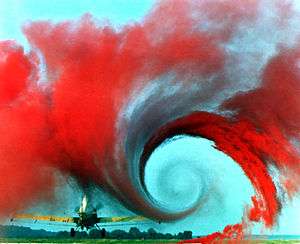
Topological mixing (or topological transitivity) means that the system evolves over time so that any given region or open set of its phase space eventually overlaps with any other given region. This mathematical concept of "mixing" corresponds to the standard intuition, and the mixing of colored dyes or fluids is an example of a chaotic system.
Topological mixing is often omitted from popular accounts of chaos, which equate chaos with only sensitivity to initial conditions. However, sensitive dependence on initial conditions alone does not give chaos. For example, consider the simple dynamical system produced by repeatedly doubling an initial value. This system has sensitive dependence on initial conditions everywhere, since any pair of nearby points eventually becomes widely separated. However, this example has no topological mixing, and therefore has no chaos. Indeed, it has extremely simple behavior: all points except 0 tend to positive or negative infinity.
Density of periodic orbits
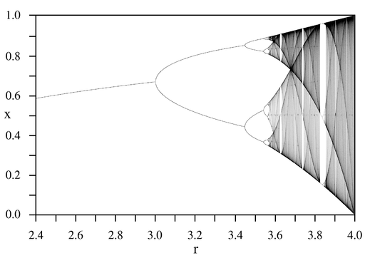
For a chaotic system to have dense periodic orbits means that every point in the space is approached arbitrarily closely by periodic orbits.[19] The one-dimensional logistic map defined by x → 4 x (1 – x) is one of the simplest systems with density of periodic orbits. For example, → → (or approximately 0.3454915 → 0.9045085 → 0.3454915) is an (unstable) orbit of period 2, and similar orbits exist for periods 4, 8, 16, etc. (indeed, for all the periods specified by Sharkovskii's theorem).[20]


Sharkovskii's theorem is the basis of the Li and Yorke[21] (1975) proof that any one-dimensional system that exhibits a regular cycle of period three will also display regular cycles of every other length, as well as completely chaotic orbits.
Strange attractors

Some dynamical systems, like the one-dimensional logistic map defined by x → 4 x (1 – x), are chaotic everywhere, but in many cases chaotic behavior is found only in a subset of phase space. The cases of most interest arise when the chaotic behavior takes place on an attractor, since then a large set of initial conditions leads to orbits that converge to this chaotic region.
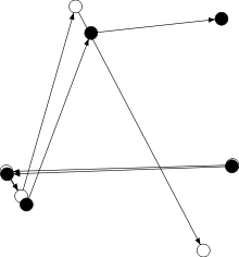
An easy way to visualize a chaotic attractor is to start with a point in the basin of attraction of the attractor, and then simply plot its subsequent orbit. Because of the topological transitivity condition, this is likely to produce a picture of the entire final attractor, and indeed both orbits shown in the figure on the right give a picture of the general shape of the Lorenz attractor. This attractor results from a simple three-dimensional model of the Lorenz weather system. The Lorenz attractor is perhaps one of the best-known chaotic system diagrams, probably because it was not only one of the first, but it is also one of the most complex and as such gives rise to a very interesting pattern, that with a little imagination, looks like the wings of a butterfly.
Unlike fixed-point attractors and limit cycles, the attractors that arise from chaotic systems, known as strange attractors, have great detail and complexity. Strange attractors occur in both continuous dynamical systems (such as the Lorenz system) and in some discrete systems (such as the Hénon map). Other discrete dynamical systems have a repelling structure called a Julia set, which forms at the boundary between basins of attraction of fixed points. Julia sets can be thought of as strange repellers. Both strange attractors and Julia sets typically have a fractal structure, and the fractal dimension can be calculated for them.
Minimum complexity of a chaotic system
Discrete chaotic systems, such as the logistic map, can exhibit strange attractors whatever their dimensionality. In contrast, for continuous dynamical systems, the Poincaré–Bendixson theorem shows that a strange attractor can only arise in three or more dimensions. Finite-dimensional linear systems are never chaotic; for a dynamical system to display chaotic behavior, it must be either nonlinear or infinite-dimensional.
The Poincaré–Bendixson theorem states that a two-dimensional differential equation has very regular behavior. The Lorenz attractor discussed above is generated by a system of three differential equations such as:

where , , and make up the system state, is time, and , , are the system parameters. Five of the terms on the right hand side are linear, while two are quadratic; a total of seven terms. Another well-known chaotic attractor is generated by the Rössler equations, which have only one nonlinear term out of seven. Sprott[22] found a three-dimensional system with just five terms, that had only one nonlinear term, which exhibits chaos for certain parameter values. Zhang and Heidel[23][24] showed that, at least for dissipative and conservative quadratic systems, three-dimensional quadratic systems with only three or four terms on the right-hand side cannot exhibit chaotic behavior. The reason is, simply put, that solutions to such systems are asymptotic to a two-dimensional surface and therefore solutions are well behaved.


While the Poincaré–Bendixson theorem shows that a continuous dynamical system on the Euclidean plane cannot be chaotic, two-dimensional continuous systems with non-Euclidean geometry can exhibit chaotic behavior.[25] Perhaps surprisingly, chaos may occur also in linear systems, provided they are infinite dimensional.[26] A theory of linear chaos is being developed in a branch of mathematical analysis known as functional analysis.
Jerk systems
In physics, jerk is the third derivative of position, with respect to time. As such, differential equations of the form

are sometimes called Jerk equations. It has been shown, that a jerk equation, which is equivalent to a system of three first order, ordinary, non-linear differential equations is in a certain sense the minimal setting for solutions showing chaotic behaviour. This motivates mathematical interest in jerk systems. Systems involving a fourth or higher derivative are called accordingly hyperjerk systems.[27]
A jerk system's behavior is described by a jerk equation, and for certain jerk equations, simple electronic circuits can model solutions. These circuits are known as jerk circuits.
One of the most interesting properties of jerk circuits is the possibility of chaotic behavior. In fact, certain well-known chaotic systems, such as the Lorenz attractor and the Rössler map, are conventionally described as a system of three first-order differential equations that can combine into a single (although rather complicated) jerk equation. Nonlinear jerk systems are in a sense minimally complex systems to show chaotic behaviour, there is no chaotic system involving only two first-order, ordinary differential equations (the system resulting in an equation of second order only).
An example of a jerk equation with nonlinearity in the magnitude of is:

Here, A is an adjustable parameter. This equation has a chaotic solution for A=3/5 and can be implemented with the following jerk circuit; the required nonlinearity is brought about by the two diodes:

In the above circuit, all resistors are of equal value, except , and all capacitors are of equal size. The dominant frequency is . The output of op amp 0 will correspond to the x variable, the output of 1 corresponds to the first derivative of x and the output of 2 corresponds to the second derivative.


Spontaneous order
Under the right conditions, chaos spontaneously evolves into a lockstep pattern. In the Kuramoto model, four conditions suffice to produce synchronization in a chaotic system. Examples include the coupled oscillation of Christiaan Huygens' pendulums, fireflies, neurons, the London Millennium Bridge resonance, and large arrays of Josephson junctions.[28]
History

An early proponent of chaos theory was Henri Poincaré. In the 1880s, while studying the three-body problem, he found that there can be orbits that are nonperiodic, and yet not forever increasing nor approaching a fixed point.[29][30] In 1898 Jacques Hadamard published an influential study of the chaotic motion of a free particle gliding frictionlessly on a surface of constant negative curvature, called "Hadamard's billiards".[31] Hadamard was able to show that all trajectories are unstable, in that all particle trajectories diverge exponentially from one another, with a positive Lyapunov exponent.
Chaos theory got its start in the field of ergodic theory. Later studies, also on the topic of nonlinear differential equations, were carried out by George David Birkhoff,[32] Andrey Nikolaevich Kolmogorov,[33][34][35] Mary Lucy Cartwright and John Edensor Littlewood,[36] and Stephen Smale.[37] Except for Smale, these studies were all directly inspired by physics: the three-body problem in the case of Birkhoff, turbulence and astronomical problems in the case of Kolmogorov, and radio engineering in the case of Cartwright and Littlewood. Although chaotic planetary motion had not been observed, experimentalists had encountered turbulence in fluid motion and nonperiodic oscillation in radio circuits without the benefit of a theory to explain what they were seeing.
Despite initial insights in the first half of the twentieth century, chaos theory became formalized as such only after mid-century, when it first became evident to some scientists that linear theory, the prevailing system theory at that time, simply could not explain the observed behavior of certain experiments like that of the logistic map. What had been attributed to measure imprecision and simple "noise" was considered by chaos theorists as a full component of the studied systems.
The main catalyst for the development of chaos theory was the electronic computer. Much of the mathematics of chaos theory involves the repeated iteration of simple mathematical formulas, which would be impractical to do by hand. Electronic computers made these repeated calculations practical, while figures and images made it possible to visualize these systems. As a graduate student in Chihiro Hayashi's laboratory at Kyoto University, Yoshisuke Ueda was experimenting with analog computers and noticed, on Nov. 27, 1961, what he called "randomly transitional phenomena". Yet his advisor did not agree with his conclusions at the time, and did not allow him to report his findings until 1970.[38][39]
Edward Lorenz was an early pioneer of the theory. His interest in chaos came about accidentally through his work on weather prediction in 1961.[8] Lorenz was using a simple digital computer, a Royal McBee LGP-30, to run his weather simulation. He wanted to see a sequence of data again, and to save time he started the simulation in the middle of its course. He did this by entering a printout of the data that corresponded to conditions in the middle of the original simulation. To his surprise, the weather the machine began to predict was completely different from the previous calculation. Lorenz tracked this down to the computer printout. The computer worked with 6-digit precision, but the printout rounded variables off to a 3-digit number, so a value like 0.506127 printed as 0.506. This difference is tiny, and the consensus at the time would have been that it should have no practical effect. However, Lorenz discovered that small changes in initial conditions produced large changes in long-term outcome.[40] Lorenz's discovery, which gave its name to Lorenz attractors, showed that even detailed atmospheric modelling cannot, in general, make precise long-term weather predictions.
In 1963, Benoit Mandelbrot found recurring patterns at every scale in data on cotton prices.[41] Beforehand he had studied information theory and concluded noise was patterned like a Cantor set: on any scale the proportion of noise-containing periods to error-free periods was a constant – thus errors were inevitable and must be planned for by incorporating redundancy.[42] Mandelbrot described both the "Noah effect" (in which sudden discontinuous changes can occur) and the "Joseph effect" (in which persistence of a value can occur for a while, yet suddenly change afterwards).[43][44] This challenged the idea that changes in price were normally distributed. In 1967, he published "How long is the coast of Britain? Statistical self-similarity and fractional dimension", showing that a coastline's length varies with the scale of the measuring instrument, resembles itself at all scales, and is infinite in length for an infinitesimally small measuring device.[45] Arguing that a ball of twine appears as a point when viewed from far away (0-dimensional), a ball when viewed from fairly near (3-dimensional), or a curved strand (1-dimensional), he argued that the dimensions of an object are relative to the observer and may be fractional. An object whose irregularity is constant over different scales ("self-similarity") is a fractal (examples include the Menger sponge, the Sierpiński gasket, and the Koch curve or snowflake, which is infinitely long yet encloses a finite space and has a fractal dimension of circa 1.2619). In 1982 Mandelbrot published The Fractal Geometry of Nature, which became a classic of chaos theory.[46] Biological systems such as the branching of the circulatory and bronchial systems proved to fit a fractal model.[47]
In December 1977, the New York Academy of Sciences organized the first symposium on Chaos, attended by David Ruelle, Robert May, James A. Yorke (coiner of the term "chaos" as used in mathematics), Robert Shaw, and the meteorologist Edward Lorenz. The following year, independently Pierre Coullet and Charles Tresser with the article "Iterations d'endomorphismes et groupe de renormalisation" and Mitchell Feigenbaum with the article "Quantitative Universality for a Class of Nonlinear Transformations" described logistic maps.[48][49] They notably discovered the universality in chaos, permitting the application of chaos theory to many different phenomena.
In 1979, Albert J. Libchaber, during a symposium organized in Aspen by Pierre Hohenberg, presented his experimental observation of the bifurcation cascade that leads to chaos and turbulence in Rayleigh–Bénard convection systems. He was awarded the Wolf Prize in Physics in 1986 along with Mitchell J. Feigenbaum for their inspiring achievements.[50]
In 1986, the New York Academy of Sciences co-organized with the National Institute of Mental Health and the Office of Naval Research the first important conference on chaos in biology and medicine. There, Bernardo Huberman presented a mathematical model of the eye tracking disorder among schizophrenics.[51] This led to a renewal of physiology in the 1980s through the application of chaos theory, for example, in the study of pathological cardiac cycles.
In 1987, Per Bak, Chao Tang and Kurt Wiesenfeld published a paper in Physical Review Letters[52] describing for the first time self-organized criticality (SOC), considered one of the mechanisms by which complexity arises in nature.
Alongside largely lab-based approaches such as the Bak–Tang–Wiesenfeld sandpile, many other investigations have focused on large-scale natural or social systems that are known (or suspected) to display scale-invariant behavior. Although these approaches were not always welcomed (at least initially) by specialists in the subjects examined, SOC has nevertheless become established as a strong candidate for explaining a number of natural phenomena, including earthquakes, (which, long before SOC was discovered, were known as a source of scale-invariant behavior such as the Gutenberg–Richter law describing the statistical distribution of earthquake sizes, and the Omori law[53] describing the frequency of aftershocks), solar flares, fluctuations in economic systems such as financial markets (references to SOC are common in econophysics), landscape formation, forest fires, landslides, epidemics, and biological evolution (where SOC has been invoked, for example, as the dynamical mechanism behind the theory of "punctuated equilibria" put forward by Niles Eldredge and Stephen Jay Gould). Given the implications of a scale-free distribution of event sizes, some researchers have suggested that another phenomenon that should be considered an example of SOC is the occurrence of wars. These investigations of SOC have included both attempts at modelling (either developing new models or adapting existing ones to the specifics of a given natural system), and extensive data analysis to determine the existence and/or characteristics of natural scaling laws.
In the same year, James Gleick published Chaos: Making a New Science, which became a best-seller and introduced the general principles of chaos theory as well as its history to the broad public, though his history under-emphasized important Soviet contributions.[54] Initially the domain of a few, isolated individuals, chaos theory progressively emerged as a transdisciplinary and institutional discipline, mainly under the name of nonlinear systems analysis. Alluding to Thomas Kuhn's concept of a paradigm shift exposed in The Structure of Scientific Revolutions (1962), many "chaologists" (as some described themselves) claimed that this new theory was an example of such a shift, a thesis upheld by Gleick.
The availability of cheaper, more powerful computers broadens the applicability of chaos theory. Currently, chaos theory remains an active area of research,[55] involving many different disciplines (mathematics, topology, physics, social systems, population modeling, biology, meteorology, astrophysics, information theory, computational neuroscience, etc.).
Distinguishing random from chaotic data
It can be difficult to tell from data whether a physical or other observed process is random or chaotic, because in practice no time series consists of a pure "signal." There is always be some form of corrupting noise, even if it is present as round-off or truncation error. Thus, any real time series, even if mostly deterministic, contains some (pseudo-)randomness.[56][57]
All methods for distinguishing deterministic and stochastic processes rely on the fact that a deterministic system always evolves in the same way from a given starting point.[56][58] Thus, given a time series to test for determinism, one can
- pick a test state;
- search the time series for a similar or nearby state; and
- compare their respective time evolutions.
Define the error as the difference between the time evolution of the test state and the time evolution of the nearby state. A deterministic system has an error that either remains small (stable, regular solution) or increases exponentially with time (chaos). A stochastic system has a randomly distributed error.[59]
Essentially, all measures of determinism taken from time series rely upon finding the closest states to a given test state (e.g., correlation dimension, Lyapunov exponents, etc.). To define the state of a system, one typically relies on phase space embedding methods such as Poincaré plots.[60] Typically one chooses an embedding dimension and investigates the propagation of the error between two nearby states. If the error looks random, one increases the dimension. If the dimension can be increased to obtain a deterministically looking error, then analysis is done. Though it may sound simple, one complication is that as the dimension increases, the search for a nearby state requires a lot more computation time and a lot of data (the amount of data required increases exponentially with embedding dimension) to find a suitably close candidate. If the embedding dimension (number of measures per state) is too small (less than the "true" value), deterministic data can appear random, but in theory there is no problem of making the dimension too large—the method still works.
When a nonlinear deterministic system is attended by external fluctuations, its trajectories present serious and permanent distortions. Furthermore, the noise is amplified due to the inherent nonlinearity and reveals totally new dynamical properties. Statistical tests attempting to separate noise from the deterministic skeleton or inversely isolate the deterministic part risk failure. Things become worse when the deterministic component is a nonlinear feedback system.[61] In presence of interactions between nonlinear deterministic components and noise, the resulting nonlinear series can display dynamics that traditional tests for nonlinearity are sometimes not able to capture.[62]
The question of how to distinguish deterministic chaotic systems from stochastic systems has also been discussed in philosophy. It has been shown that they might be observationally equivalent.[63]
Applications

Chaos theory was born from observing weather patterns, but it has become applicable to a variety of other situations. Some areas benefiting from chaos theory today are geology, mathematics, microbiology, biology, computer science, economics,[65][66][67] engineering,[68] finance,[69][70] algorithmic trading,[71][72][73] meteorology, philosophy, physics, politics, population dynamics,[74] psychology,[10] and robotics. A few categories are listed below with examples, but this is by no means a comprehensive list as new applications are appearing.
Computer science
Chaos theory is not new to computer science and has been used for many years in cryptography. One type of encryption, secret key or symmetric key, relies on diffusion and confusion, which is modeled well by chaos theory.[75] Another type of computing, DNA computing, when paired with chaos theory, offers a more efficient way to encrypt images and other information.[76] Robotics is another area that has recently benefited from chaos theory. Instead of robots acting in a trial-and-error type of refinement to interact with their environment, chaos theory has been used to build a predictive model.[77] Chaotic dynamics have been exhibited by passive walking biped robots.[78]
Biology
For over a hundred years, biologists have been keeping track of populations of different species with population models. Most models are continuous, but recently scientists have been able to implement chaotic models in certain populations.[79] For example, a study on models of Canadian lynx showed there was chaotic behavior in the population growth.[80] Chaos can also be found in ecological systems, such as hydrology. While a chaotic model for hydrology has its shortcomings, there is still much to learn from looking at the data through the lens of chaos theory.[81] Another biological application is found in cardiotocography. Fetal surveillance is a delicate balance of obtaining accurate information while being as noninvasive as possible. Better models of warning signs of fetal hypoxia can be obtained through chaotic modeling.[82]
Other areas
In chemistry, predicting gas solubility is essential to manufacturing polymers, but models using particle swarm optimization (PSO) tend to converge to the wrong points. An improved version of PSO has been created by introducing chaos, which keeps the simulations from getting stuck.[83] In celestial mechanics, especially when observing asteroids, applying chaos theory leads to better predictions about when these objects will approach Earth and other planets.[84] Four of the five moons of Pluto rotate chaotically. In quantum physics and electrical engineering, the study of large arrays of Josephson junctions benefitted greatly from chaos theory.[85] Closer to home, coal mines have always been dangerous places where frequent natural gas leaks cause many deaths. Until recently, there was no reliable way to predict when they would occur. But these gas leaks have chaotic tendencies that, when properly modeled, can be predicted fairly accurately.[86]
Chaos theory can be applied outside of the natural sciences. By adapting a model of career counseling to include a chaotic interpretation of the relationship between employees and the job market, better suggestions can be made to people struggling with career decisions.[87] Modern organizations are increasingly seen as open complex adaptive systems with fundamental natural nonlinear structures, subject to internal and external forces that may contribute chaos. The chaos metaphor—used in verbal theories—grounded on mathematical models and psychological aspects of human behavior provides helpful insights to describing the complexity of small work groups, that go beyond the metaphor itself.[88]

It is possible that economic models can also be improved through an application of chaos theory, but predicting the health of an economic system and what factors influence it most is an extremely complex task.[89] Economic and financial systems are fundamentally different from those in the classical natural sciences since the former are inherently stochastic in nature, as they result from the interactions of people, and thus pure deterministic models are unlikely to provide accurate representations of the data. The empirical literature that tests for chaos in economics and finance presents very mixed results, in part due to confusion between specific tests for chaos and more general tests for non-linear relationships.[90]
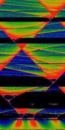
Traffic forecasting also benefits from applications of chaos theory. Better predictions of when traffic will occur lets measures be taken to disperse it before it would have occurred. Combining chaos theory principles with a few other methods has led to a more accurate short-term prediction model (see the plot of the BML traffic model at right).[91]
Chaos theory can be applied in psychology. For example, in modeling group behavior in which heterogeneous members may behave as if sharing to different degrees what in Wilfred Bion's theory is a basic assumption, the group dynamics is the result of the individual dynamics of the members: each individual reproduces the group dynamics in a different scale, and the chaotic behavior of the group is reflected in each member.[92]
See also
- Examples of chaotic systems
- Advected contours
- Arnold's cat map
- Bouncing ball dynamics
- Chua's circuit
- Cliodynamics
- Coupled map lattice
- Double pendulum
- Duffing equation
- Dynamical billiards
- Economic bubble
- Gaspard-Rice system
- Hénon map
- Horseshoe map
- List of chaotic maps
- Logistic map
- Rössler attractor
- Standard map
- Swinging Atwood's machine
- Tilt A Whirl
- Other related topics
- Amplitude death
- Anosov diffeomorphism
- Bifurcation theory
- Catastrophe theory
- Chaos theory in organizational development
- Chaotic mixing
- Chaotic scattering
- Complexity
- Control of chaos
- Edge of chaos
- Emergence
- Fractal
- Kolmogorov–Arnold–Moser theorem
- Ill-conditioning
- Ill-posedness
- Nonlinear system
- Patterns in nature
- Predictability
- Quantum chaos
- Santa Fe Institute
- Synchronization of chaos
- Unintended consequence
- People
- Ralph Abraham
- Michael Berry
- Leon O. Chua
- Ivar Ekeland
- Doyne Farmer
- Mitchell Feigenbaum
- Martin Gutzwiller
- Brosl Hasslacher
- Michel Hénon
- Andrey Nikolaevich Kolmogorov
- Edward Lorenz
- Aleksandr Lyapunov
- Ian Malcolm (Jurassic Park character)
- Benoit Mandelbrot
- Norman Packard
- Henri Poincaré
- Otto Rössler
- David Ruelle
- Oleksandr Mikolaiovich Sharkovsky
- Robert Shaw
- Floris Takens
- James A. Yorke
- George M. Zaslavsky
References
- ↑ Boeing (2015). "Chaos Theory and the Logistic Map". Retrieved 2015-07-16.
- ↑ Kellert, Stephen H. (1993). In the Wake of Chaos: Unpredictable Order in Dynamical Systems. University of Chicago Press. p. 32. ISBN 0-226-42976-8.
- 1 2 Boeing, G. (2016). "Visual Analysis of Nonlinear Dynamical Systems: Chaos, Fractals, Self-Similarity and the Limits of Prediction". Systems. 4 (4): 37. doi:10.3390/systems4040037. Retrieved 2016-12-02.
- ↑ Kellert 1993, p. 56
- ↑ Kellert 1993, p. 62
- 1 2 Werndl, Charlotte (2009). "What are the New Implications of Chaos for Unpredictability?". The British Journal for the Philosophy of Science. 60 (1): 195–220. doi:10.1093/bjps/axn053.
- ↑ Danforth, Christopher M. (April 2013). "Chaos in an Atmosphere Hanging on a Wall". Mathematics of Planet Earth 2013. Retrieved 4 April 2013.
- 1 2 Lorenz, Edward N. (1963). "Deterministic non-periodic flow". Journal of the Atmospheric Sciences. 20 (2): 130–141. Bibcode:1963JAtS...20..130L. doi:10.1175/1520-0469(1963)020<0130:DNF>2.0.CO;2.
- ↑ Ivancevic, Vladimir G.; Tijana T. Ivancevic (2008). Complex nonlinearity: chaos, phase transitions, topology change, and path integrals. Springer. ISBN 978-3-540-79356-4.
- 1 2 Safonov, Leonid A.; Tomer, Elad; Strygin, Vadim V.; Ashkenazy, Yosef; Havlin, Shlomo (2002). "Multifractal chaotic attractors in a system of delay-differential equations modeling road traffic". Chaos: An Interdisciplinary Journal of Nonlinear Science. 12 (4): 1006. Bibcode:2002Chaos..12.1006S. doi:10.1063/1.1507903. ISSN 1054-1500.
- ↑ Sync: The Emerging Science of Spontaneous Order, Steven Strogatz, Hyperion, New York, 2003, pages 189-190.
- ↑ Definition of chaos at Wiktionary;
- ↑ Hasselblatt, Boris; Anatole Katok (2003). A First Course in Dynamics: With a Panorama of Recent Developments. Cambridge University Press. ISBN 0-521-58750-6.
- ↑ Elaydi, Saber N. (1999). Discrete Chaos. Chapman & Hall/CRC. p. 117. ISBN 1-58488-002-3.
- ↑ Basener, William F. (2006). Topology and its applications. Wiley. p. 42. ISBN 0-471-68755-3.
- ↑ Vellekoop, Michel; Berglund, Raoul (April 1994). "On Intervals, Transitivity = Chaos". The American Mathematical Monthly. 101 (4): 353–5. doi:10.2307/2975629. JSTOR 2975629.
- ↑ Medio, Alfredo; Lines, Marji (2001). Nonlinear Dynamics: A Primer. Cambridge University Press. p. 165. ISBN 0-521-55874-3.
- ↑ Watts, Robert G. (2007). Global Warming and the Future of the Earth. Morgan & Claypool. p. 17.
- ↑ Devaney 2003
- ↑ Alligood, Sauer & Yorke 1997
- ↑ Li, T.Y.; Yorke, J.A. (1975). "Period Three Implies Chaos" (PDF). American Mathematical Monthly. 82 (10): 985–92. Bibcode:1975AmMM...82..985L. doi:10.2307/2318254. Archived from the original (PDF) on 2009-12-29.
- ↑ Sprott, J.C. (1997). "Simplest dissipative chaotic flow". Physics Letters A. 228 (4–5): 271–274. Bibcode:1997PhLA..228..271S. doi:10.1016/S0375-9601(97)00088-1.
- ↑ Fu, Z.; Heidel, J. (1997). "Non-chaotic behaviour in three-dimensional quadratic systems". Nonlinearity. 10 (5): 1289–1303. Bibcode:1997Nonli..10.1289F. doi:10.1088/0951-7715/10/5/014.
- ↑ Heidel, J.; Fu, Z. (1999). "Nonchaotic behaviour in three-dimensional quadratic systems II. The conservative case". Nonlinearity. 12 (3): 617–633. Bibcode:1999Nonli..12..617H. doi:10.1088/0951-7715/12/3/012.
- ↑ Rosario, Pedro (2006). Underdetermination of Science: Part I. Lulu.com. ISBN 1411693914.
- ↑ Bonet, J.; Martínez-Giménez, F.; Peris, A. (2001). "A Banach space which admits no chaotic operator". Bulletin of the London Mathematical Society. 33 (2): 196–8. doi:10.1112/blms/33.2.196.
- ↑ K. E. Chlouverakis and J. C. Sprott, Chaos Solitons & Fractals 28, 739-746 (2005), Chaotic Hyperjerk Systems, http://sprott.physics.wisc.edu/pubs/paper297.htm
- ↑ Steven Strogatz, Sync: The Emerging Science of Spontaneous Order, Hyperion, 2003.
- ↑ Poincaré, Jules Henri (1890). "Sur le problème des trois corps et les équations de la dynamique. Divergence des séries de M. Lindstedt". Acta Mathematica. 13: 1–270. doi:10.1007/BF02392506.
- ↑ Diacu, Florin; Holmes, Philip (1996). Celestial Encounters: The Origins of Chaos and Stability. Princeton University Press.
- ↑ Hadamard, Jacques (1898). "Les surfaces à courbures opposées et leurs lignes géodesiques". Journal de Mathématiques Pures et Appliquées. 4: 27–73.
- ↑ George D. Birkhoff, Dynamical Systems, vol. 9 of the American Mathematical Society Colloquium Publications (Providence, Rhode Island: American Mathematical Society, 1927)
- ↑ Kolmogorov, Andrey Nikolaevich (1941). "Local structure of turbulence in an incompressible fluid for very large Reynolds numbers". Doklady Akademii Nauk SSSR. 30 (4): 301–5. Bibcode:1941DoSSR..30..301K. Reprinted in: Kolmogorov, A. N. (1991). "The Local Structure of Turbulence in Incompressible Viscous Fluid for Very Large Reynolds Numbers". Proceedings of the Royal Society A. 434 (1890): 9–13. Bibcode:1991RSPSA.434....9K. doi:10.1098/rspa.1991.0075.
- ↑ Kolmogorov, A. N. (1941). "On degeneration of isotropic turbulence in an incompressible viscous liquid". Doklady Akademii Nauk SSSR. 31 (6): 538–540. Reprinted in: Kolmogorov, A. N. (1991). "Dissipation of Energy in the Locally Isotropic Turbulence". Proceedings of the Royal Society A. 434 (1890): 15–17. Bibcode:1991RSPSA.434...15K. doi:10.1098/rspa.1991.0076.
- ↑ Kolmogorov, A. N. (1954). "Preservation of conditionally periodic movements with small change in the Hamiltonian function". Doklady Akademii Nauk SSSR. Lecture Notes in Physics. 98: 527–530. Bibcode:1979LNP....93...51K. doi:10.1007/BFb0021737. ISBN 3-540-09120-3. See also Kolmogorov–Arnold–Moser theorem
- ↑ Cartwright, Mary L.; Littlewood, John E. (1945). "On non-linear differential equations of the second order, I: The equation y" + k(1−y2)y' + y = bλkcos(λt + a), k large". Journal of the London Mathematical Society. 20 (3): 180–9. doi:10.1112/jlms/s1-20.3.180. See also: Van der Pol oscillator
- ↑ Smale, Stephen (January 1960). "Morse inequalities for a dynamical system". Bulletin of the American Mathematical Society. 66: 43–49. doi:10.1090/S0002-9904-1960-10386-2.
- ↑ Abraham & Ueda 2001, See Chapters 3 and 4
- ↑ Sprott 2003, p. 89
- ↑ Gleick, James (1987). Chaos: Making a New Science. London: Cardinal. p. 17. ISBN 0-434-29554-X.
- ↑ Mandelbrot, Benoît (1963). "The variation of certain speculative prices". Journal of Business. 36 (4): 394–419. doi:10.1086/294632. JSTOR 2350970.
- ↑ Berger J.M.; Mandelbrot B. (1963). "A new model for error clustering in telephone circuits". IBM Journal of Research and Development. 7: 224–236. doi:10.1147/rd.73.0224.
- ↑ Mandelbrot, B. (1977). The Fractal Geometry of Nature. New York: Freeman. p. 248.
- ↑ See also: Mandelbrot, Benoît B.; Hudson, Richard L. (2004). The (Mis)behavior of Markets: A Fractal View of Risk, Ruin, and Reward. New York: Basic Books. p. 201.
- ↑ Mandelbrot, Benoît (5 May 1967). "How Long Is the Coast of Britain? Statistical Self-Similarity and Fractional Dimension". Science. 156 (3775): 636–8. Bibcode:1967Sci...156..636M. doi:10.1126/science.156.3775.636. PMID 17837158.
- ↑ Mandelbrot, B. (1982). The Fractal Geometry of Nature. New York: Macmillan. ISBN 0716711869.
- ↑ Buldyrev, S.V.; Goldberger, A.L.; Havlin, S.; Peng, C.K.; Stanley, H.E. (1994). "Fractals in Biology and Medicine: From DNA to the Heartbeat". In Bunde, Armin; Havlin, Shlomo. Fractals in Science. Springer. pp. 49–89. ISBN 3-540-56220-6.
- ↑ Feigenbaum, Mitchell (July 1978). "Quantitative universality for a class of nonlinear transformations". Journal of Statistical Physics. 19 (1): 25–52. Bibcode:1978JSP....19...25F. doi:10.1007/BF01020332.
- ↑ Coullet, Pierre, and Charles Tresser. "Iterations d'endomorphismes et groupe de renormalisation." Le Journal de Physique Colloques 39.C5 (1978): C5-25
- ↑ "The Wolf Prize in Physics in 1986.".
- ↑ Huberman, B.A. (July 1987). "A Model for Dysfunctions in Smooth Pursuit Eye Movement". Annals of the New York Academy of Sciences. 504 Perspectives in Biological Dynamics and Theoretical Medicine: 260–273. Bibcode:1987NYASA.504..260H. doi:10.1111/j.1749-6632.1987.tb48737.x.
- ↑ Bak, Per; Tang, Chao; Wiesenfeld, Kurt; Tang; Wiesenfeld (27 July 1987). "Self-organized criticality: An explanation of the 1/f noise". Physical Review Letters. 59 (4): 381–4. Bibcode:1987PhRvL..59..381B. doi:10.1103/PhysRevLett.59.381. However, the conclusions of this article have been subject to dispute. "?". Archived from the original on 2007-12-14.. See especially: Laurson, Lasse; Alava, Mikko J.; Zapperi, Stefano (15 September 2005). "Letter: Power spectra of self-organized critical sand piles". Journal of Statistical Mechanics: Theory and Experiment. 0511. L001.
- ↑ Omori, F. (1894). "On the aftershocks of earthquakes". Journal of the College of Science, Imperial University of Tokyo. 7: 111–200.
- ↑ Gleick, James (August 26, 2008). Chaos: Making a New Science. Penguin Books. ISBN 0143113453.
- ↑ Motter, A. E.; Campbell, D. K. (2013). "Chaos at fifty". Phys. Today. 66 (5): 27–33. doi:10.1063/pt.3.1977.
- 1 2 Provenzale, A.; Smith; Vio; Murante; et al. (1992). "Distinguishing between low-dimensional dynamics and randomness in measured time-series". Physica D. 58: 31–49. Bibcode:1992PhyD...58...31P. doi:10.1016/0167-2789(92)90100-2.
- ↑ Brock, W.A. (October 1986). "Distinguishing random and deterministic systems: Abridged version". Journal of Economic Theory. 40: 168–195. doi:10.1016/0022-0531(86)90014-1.
- ↑ Sugihara G., May R.; May (1990). "Nonlinear forecasting as a way of distinguishing chaos from measurement error in time series" (PDF). Nature. 344 (6268): 734–741. Bibcode:1990Natur.344..734S. doi:10.1038/344734a0. PMID 2330029.
- ↑ Casdagli, Martin (1991). "Chaos and Deterministic versus Stochastic Non-linear Modelling". Journal of the Royal Statistical Society, Series B. 54 (2): 303–328. JSTOR 2346130.
- ↑ Broomhead, D.S.; King, G.P.; King (June–July 1986). "Extracting qualitative dynamics from experimental data". Physica D. 20 (2–3): 217–236. Bibcode:1986PhyD...20..217B. doi:10.1016/0167-2789(86)90031-X.
- ↑ Kyrtsou C (2008). "Re-examining the sources of heteroskedasticity: the paradigm of noisy chaotic models". Physica A. 387 (27): 6785–9. Bibcode:2008PhyA..387.6785K. doi:10.1016/j.physa.2008.09.008.
- ↑ Kyrtsou, C. (2005). "Evidence for neglected linearity in noisy chaotic models". International Journal of Bifurcation and Chaos. 15 (10): 3391–4. Bibcode:2005IJBC...15.3391K. doi:10.1142/S0218127405013964.
- ↑ Werndl, Charlotte (2009). "Are Deterministic Descriptions and Indeterministic Descriptions Observationally Equivalent?". Studies in History and Philosophy of Modern Physics. 40 (3): 232–242. doi:10.1016/j.shpsb.2009.06.004.
- ↑ Stephen Coombes (February 2009). "The Geometry and Pigmentation of Seashells" (PDF). www.maths.nottingham.ac.uk. University of Nottingham. Retrieved 2013-04-10.
- ↑ Kyrtsou C.; Labys W. (2006). "Evidence for chaotic dependence between US inflation and commodity prices". Journal of Macroeconomics. 28 (1): 256–266. doi:10.1016/j.jmacro.2005.10.019.
- ↑ Kyrtsou C., Labys W.; Labys (2007). "Detecting positive feedback in multivariate time series: the case of metal prices and US inflation". Physica A. 377 (1): 227–229. Bibcode:2007PhyA..377..227K. doi:10.1016/j.physa.2006.11.002.
- ↑ Kyrtsou, C.; Vorlow, C. (2005). "Complex dynamics in macroeconomics: A novel approach". In Diebolt, C.; Kyrtsou, C. New Trends in Macroeconomics. Springer Verlag.
- ↑ Applying Chaos Theory to Embedded Applications
- ↑ Hristu-Varsakelis, D.; Kyrtsou, C. (2008). "Evidence for nonlinear asymmetric causality in US inflation, metal and stock returns". Discrete Dynamics in Nature and Society. 2008: 1–7. doi:10.1155/2008/138547. 138547.
- ↑ Kyrtsou, C.; M. Terraza, (2003). "Is it possible to study chaotic and ARCH behaviour jointly? Application of a noisy Mackey-Glass equation with heteroskedastic errors to the Paris Stock Exchange returns series". Computational Economics. 21 (3): 257–276. doi:10.1023/A:1023939610962.
- ↑ Williams, Bill Williams, Justine (2004). Trading chaos : maximize profits with proven technical techniques (2nd ed.). New York: Wiley. ISBN 9780471463085.
- ↑ Peters, Edgar E. (1994). Fractal market analysis : applying chaos theory to investment and economics (2. print. ed.). New York u.a.: Wiley. ISBN 978-0471585244.
- ↑ Peters, / Edgar E. (1996). Chaos and order in the capital markets : a new view of cycles, prices, and market volatility (2nd ed.). New York: John Wiley & Sons. ISBN 978-0471139386.
- ↑ Dilão, R.; Domingos, T. (2001). "Periodic and Quasi-Periodic Behavior in Resource Dependent Age Structured Population Models". Bulletin of Mathematical Biology. 63 (2): 207–230. doi:10.1006/bulm.2000.0213. PMID 11276524.
- ↑ Wang, Xingyuan; Zhao, Jianfeng (2012). "An improved key agreement protocol based on chaos". Commun. Nonlinear Sci. Numer. Simul. 15 (12): 4052–4057. Bibcode:2010CNSNS..15.4052W. doi:10.1016/j.cnsns.2010.02.014.
- ↑ Babaei, Majid (2013). "A novel text and image encryption method based on chaos theory and DNA computing". Natural Computing. an International Journal. 12 (1): 101–107. doi:10.1007/s11047-012-9334-9.
- ↑ Nehmzow, Ulrich; Keith Walker (Dec 2005). "Quantitative description of robot–environment interaction using chaos theory". Robotics and Autonomous Systems. 53 (3–4): 177–193. doi:10.1016/j.robot.2005.09.009.
- ↑ Goswami, Ambarish; Thuilot, Benoit; Espiau, Bernard (1998). "A Study of the Passive Gait of a Compass-Like Biped Robot: Symmetry and Chaos". The International Journal of Robotics Research. 17 (12): 1282–1301. doi:10.1177/027836499801701202.
- ↑ Eduardo, Liz; Ruiz-Herrera, Alfonso (2012). "Chaos in discrete structured population models". SIAM Journal on Applied Dynamical Systems. 11 (4): 1200–1214. doi:10.1137/120868980.
- ↑ Lai, Dejian (1996). "Comparison study of AR models on the Canadian lynx data: a close look at BDS statistic". Computational Statistics \& Data Analysis. 22 (4): 409–423. doi:10.1016/0167-9473(95)00056-9.
- ↑ Sivakumar, B (31 January 2000). "Chaos theory in hydrology: important issues and interpretations". Journal of Hydrology. 227 (1–4): 1–20. Bibcode:2000JHyd..227....1S. doi:10.1016/S0022-1694(99)00186-9.
- ↑ Bozóki, Zsolt (February 1997). "Chaos theory and power spectrum analysis in computerized cardiotocography". European Journal of Obstetrics & Gynecology and Reproductive Biology. 71 (2): 163–168. doi:10.1016/s0301-2115(96)02628-0.
- ↑ Li, Mengshan; Xingyuan Huanga; Hesheng Liua; Bingxiang Liub; Yan Wub; Aihua Xiongc; Tianwen Dong (25 October 2013). "Prediction of gas solubility in polymers by back propagation artificial neural network based on self-adaptive particle swarm optimization algorithm and chaos theory". Fluid Phase Equilibria. 356: 11–17. doi:10.1016/j.fluid.2013.07.017.
- ↑ Morbidelli, A. (2001). "Chaotic diffusion in celestial mechanics". Regular & Chaotic Dynamics. 6 (4): 339–353. doi:10.1070/rd2001v006n04abeh000182.
- ↑ Steven Strogatz, Sync: The Emerging Science of Spontaneous Order, Hyperion, 2003
- ↑ Dingqi, Li; Yuanping Chenga; Lei Wanga; Haifeng Wanga; Liang Wanga; Hongxing Zhou (May 2011). "Prediction method for risks of coal and gas outbursts based on spatial chaos theory using gas desorption index of drill cuttings". Mining Science and Technology. 21 (3): 439–443.
- ↑ Pryor, Robert G. L.; Norman E. Aniundson; Jim E. H. Bright (June 2008). "Probabilities and Possibilities: The Strategic Counseling Implications of the Chaos Theory of Careers". The Career Development Quarterly. 56: 309–318. doi:10.1002/j.2161-0045.2008.tb00096.x.
- ↑ Dal Forno, Arianna; Merlone, Ugo (2013). "Chaotic Dynamics in Organization Theory". In Bischi, Gian Italo; Chiarella, Carl; Shusko, Irina. Global Analysis of Dynamic Models in Economics and Finance. Springer-Verlag. pp. 185–204. ISBN 978-3-642-29503-4.
- ↑ Juárez, Fernando (2011). "Applying the theory of chaos and a complex model of health to establish relations among financial indicators". Procedia Computer Science. 3: 982–986. doi:10.1016/j.procs.2010.12.161.
- ↑ Brooks, Chris (1998). "Chaos in foreign exchange markets: a sceptical view". Computational Economics. 11: 265–281. doi:10.1023/A:1008650024944. ISSN 1572-9974.
- ↑ Wang, Jin; Qixin Shi (February 2013). "Short-term traffic speed forecasting hybrid model based on Chaos–Wavelet Analysis-Support Vector Machine theory". Transportation Research Part C: Emerging Technologies. 27: 219–232. doi:10.1016/j.trc.2012.08.004.
- ↑ Dal Forno, Arianna; Merlone, Ugo (2013). "Nonlinear dynamics in work groups with Bion's basic assumptions". Nonlinear Dynamics, Psychology, and Life Sciences. 17 (2): 295–315. ISSN 1090-0578.
Scientific literature
Articles
- Sharkovskii, A.N. (1964). "Co-existence of cycles of a continuous mapping of the line into itself". Ukrainian Math. J. 16: 61–71.
- Li, T.Y.; Yorke, J.A. (1975). "Period Three Implies Chaos". American Mathematical Monthly. 82 (10): 985–92. Bibcode:1975AmMM...82..985L. doi:10.2307/2318254.
- Crutchfield; Tucker; Morrison; J.D.; Packard; N.H.; Shaw; R.S (December 1986). "Chaos". Scientific American. 255 (6): 38–49 (bibliography p.136). Bibcode:1986SciAm.255...38T. Online version (Note: the volume and page citation cited for the online text differ from that cited here. The citation here is from a photocopy, which is consistent with other citations found online that don't provide article views. The online content is identical to the hardcopy text. Citation variations are related to country of publication).
- Kolyada, S.F. (2004). "Li-Yorke sensitivity and other concepts of chaos". Ukrainian Math. J. 56 (8): 1242–57. doi:10.1007/s11253-005-0055-4.
- Strelioff, C.; Hübler, A. (2006). "Medium-Term Prediction of Chaos" (PDF). Phys. Rev. Lett. 96 (4): 044101. Bibcode:2006PhRvL..96d4101S. doi:10.1103/PhysRevLett.96.044101. PMID 16486826. 044101. Archived from the original (PDF) on 2013-04-26.
- Hübler, A.; Foster, G.; Phelps, K. (2007). "Managing Chaos: Thinking out of the Box" (PDF). Complexity. 12 (3): 10–13. doi:10.1002/cplx.20159.
- Motter, Adilson E.; Campbell, David K. (2013). "Chaos at 50". Physics Today. 66: 27. doi:10.1063/PT.3.1977.
- Boeing, G. (2016). "Visual Analysis of Nonlinear Dynamical Systems: Chaos, Fractals, Self-Similarity and the Limits of Prediction". Systems. 4 (4): 37. doi:10.3390/systems4040037.
Textbooks
- Alligood, K.T.; Sauer, T.; Yorke, J.A. (1997). Chaos: an introduction to dynamical systems. Springer-Verlag. ISBN 0-387-94677-2.
- Baker, G. L. (1996). Chaos, Scattering and Statistical Mechanics. Cambridge University Press. ISBN 0-521-39511-9.
- Badii, R.; Politi A. (1997). Complexity: hierarchical structures and scaling in physics. Cambridge University Press. ISBN 0-521-66385-7.
- Bunde; Havlin, Shlomo, eds. (1996). Fractals and Disordered Systems. Springer. ISBN 3642848702. and Bunde; Havlin, Shlomo, eds. (1994). Fractals in Science. Springer. ISBN 3-540-56220-6.
- Collet, Pierre, and Eckmann, Jean-Pierre (1980). Iterated Maps on the Interval as Dynamical Systems. Birkhauser. ISBN 0-8176-4926-3.
- Devaney, Robert L. (2003). An Introduction to Chaotic Dynamical Systems (2nd ed.). Westview Press. ISBN 0-8133-4085-3.
- Gollub, J. P.; Baker, G. L. (1996). Chaotic dynamics. Cambridge University Press. ISBN 0-521-47685-2.
- Guckenheimer, John; Holmes, Philip (1983). Nonlinear Oscillations, Dynamical Systems, and Bifurcations of Vector Fields. Springer-Verlag. ISBN 0-387-90819-6.
- Gulick, Denny (1992). Encounters with Chaos. McGraw-Hill. ISBN 0-07-025203-3.
- Gutzwiller, Martin (1990). Chaos in Classical and Quantum Mechanics. Springer-Verlag. ISBN 0-387-97173-4.
- Hoover, William Graham (2001) [1999]. Time Reversibility, Computer Simulation, and Chaos. World Scientific. ISBN 981-02-4073-2.
- Kautz, Richard (2011). Chaos: The Science of Predictable Random Motion. Oxford University Press. ISBN 978-0-19-959458-0.
- Kiel, L. Douglas; Elliott, Euel W. (1997). Chaos Theory in the Social Sciences. Perseus Publishing. ISBN 0-472-08472-0.
- Moon, Francis (1990). Chaotic and Fractal Dynamics. Springer-Verlag. ISBN 0-471-54571-6.
- Ott, Edward (2002). Chaos in Dynamical Systems. Cambridge University Press. ISBN 0-521-01084-5.
- Strogatz, Steven (2000). Nonlinear Dynamics and Chaos. Perseus Publishing. ISBN 0-7382-0453-6.
- Sprott, Julien Clinton (2003). Chaos and Time-Series Analysis. Oxford University Press. ISBN 0-19-850840-9.
- Tél, Tamás; Gruiz, Márton (2006). Chaotic dynamics: An introduction based on classical mechanics. Cambridge University Press. ISBN 0-521-83912-2.
- Teschl, Gerald (2012). Ordinary Differential Equations and Dynamical Systems. Providence: American Mathematical Society. ISBN 978-0-8218-8328-0.
- Thompson JM, Stewart HB (2001). Nonlinear Dynamics And Chaos. John Wiley and Sons Ltd. ISBN 0-471-87645-3.
- Tufillaro; Reilly (1992). An experimental approach to nonlinear dynamics and chaos. Addison-Wesley. ISBN 0-201-55441-0.
- Wiggins, Stephen (2003). Introduction to Applied Dynamical Systems and Chaos. Springer. ISBN 0-387-00177-8.
- Zaslavsky, George M. (2005). Hamiltonian Chaos and Fractional Dynamics. Oxford University Press. ISBN 0-19-852604-0.
Semitechnical and popular works
- Christophe Letellier, Chaos in Nature, World Scientific Publishing Company, 2012, ISBN 978-981-4374-42-2.
- Abraham, Ralph H.; Ueda, Yoshisuke, eds. (2000). The Chaos Avant-Garde: Memoirs of the Early Days of Chaos Theory. World Scientific. ISBN 978-981-238-647-2.
- Barnsley, Michael F. (2000). Fractals Everywhere. Morgan Kaufmann. ISBN 978-0-12-079069-2.
- Bird, Richard J. (2003). Chaos and Life: Complexit and Order in Evolution and Thought. Columbia University Press. ISBN 978-0-231-12662-5.
- John Briggs and David Peat, Turbulent Mirror: : An Illustrated Guide to Chaos Theory and the Science of Wholeness, Harper Perennial 1990, 224 pp.
- John Briggs and David Peat, Seven Life Lessons of Chaos: Spiritual Wisdom from the Science of Change, Harper Perennial 2000, 224 pp.
- Cunningham, Lawrence A. (1994). "From Random Walks to Chaotic Crashes: The Linear Genealogy of the Efficient Capital Market Hypothesis". George Washington Law Review. 62: 546.
- Predrag Cvitanović, Universality in Chaos, Adam Hilger 1989, 648 pp.
- Leon Glass and Michael C. Mackey, From Clocks to Chaos: The Rhythms of Life, Princeton University Press 1988, 272 pp.
- James Gleick, Chaos: Making a New Science, New York: Penguin, 1988. 368 pp.
- John Gribbin. Deep Simplicity. Penguin Press Science. Penguin Books.
- L Douglas Kiel, Euel W Elliott (ed.), Chaos Theory in the Social Sciences: Foundations and Applications, University of Michigan Press, 1997, 360 pp.
- Arvind Kumar, Chaos, Fractals and Self-Organisation; New Perspectives on Complexity in Nature , National Book Trust, 2003.
- Hans Lauwerier, Fractals, Princeton University Press, 1991.
- Edward Lorenz, The Essence of Chaos, University of Washington Press, 1996.
- Alan Marshall (2002) The Unity of Nature: Wholeness and Disintegration in Ecology and Science, Imperial College Press: London
- Heinz-Otto Peitgen and Dietmar Saupe (Eds.), The Science of Fractal Images, Springer 1988, 312 pp.
- Clifford A. Pickover, Computers, Pattern, Chaos, and Beauty: Graphics from an Unseen World , St Martins Pr 1991.
- Ilya Prigogine and Isabelle Stengers, Order Out of Chaos, Bantam 1984.
- Heinz-Otto Peitgen and P. H. Richter, The Beauty of Fractals : Images of Complex Dynamical Systems, Springer 1986, 211 pp.
- David Ruelle, Chance and Chaos, Princeton University Press 1993.
- Ivars Peterson, Newton's Clock: Chaos in the Solar System, Freeman, 1993.
- Ian Roulstone; John Norbury (2013). Invisible in the Storm: the role of mathematics in understanding weather. Princeton University Press. ISBN 0691152721.
- David Ruelle, Chaotic Evolution and Strange Attractors, Cambridge University Press, 1989.
- Peter Smith, Explaining Chaos, Cambridge University Press, 1998.
- Ian Stewart, Does God Play Dice?: The Mathematics of Chaos , Blackwell Publishers, 1990.
- Steven Strogatz, Sync: The emerging science of spontaneous order, Hyperion, 2003.
- Yoshisuke Ueda, The Road To Chaos, Aerial Pr, 1993.
- M. Mitchell Waldrop, Complexity : The Emerging Science at the Edge of Order and Chaos, Simon & Schuster, 1992.
- Sawaya, Antonio (2010). Financial time series analysis : Chaos and neurodynamics approach.
External links
| Wikimedia Commons has media related to Chaos theory. |
- Hazewinkel, Michiel, ed. (2001), "Chaos", Encyclopedia of Mathematics, Springer, ISBN 978-1-55608-010-4
- Nonlinear Dynamics Research Group with Animations in Flash
- The Chaos group at the University of Maryland
- The Chaos Hypertextbook. An introductory primer on chaos and fractals
- ChaosBook.org An advanced graduate textbook on chaos (no fractals)
- Society for Chaos Theory in Psychology & Life Sciences
- Nonlinear Dynamics Research Group at CSDC, Florence Italy
- Interactive live chaotic pendulum experiment, allows users to interact and sample data from a real working damped driven chaotic pendulum
- Nonlinear dynamics: how science comprehends chaos, talk presented by Sunny Auyang, 1998.
- Nonlinear Dynamics. Models of bifurcation and chaos by Elmer G. Wiens
- Gleick's Chaos (excerpt)
- Systems Analysis, Modelling and Prediction Group at the University of Oxford
- A page about the Mackey-Glass equation
- High Anxieties — The Mathematics of Chaos (2008) BBC documentary directed by David Malone
- The chaos theory of evolution - article published in Newscientist featuring similarities of evolution and non-linear systems including fractal nature of life and chaos.
- Jos Leys, Étienne Ghys et Aurélien Alvarez, Chaos, A Mathematical Adventure. Nine films about dynamical systems, the butterfly effect and chaos theory, intended for a wide audience.
| Chaos theory | 
 | |
|---|---|---|
| Chaotic maps (list) |
| |
| Chaos systems | ||
| Chaos theorists | ||
| Patterns | .jpg) | |
|---|---|---|
| Causes | ||
| People | ||
| Related | ||