Capital asset pricing model

An estimation of the CAPM and the security market line (purple) for the Dow Jones Industrial Average over 3 years for monthly data.

In finance, the capital asset pricing model (CAPM) is a model used to determine a theoretically appropriate required rate of return of an asset, to make decisions about adding assets to a well-diversified portfolio.

Overview

The model takes into account the asset's sensitivity to non-diversifiable risk (also known as systematic risk or market risk), often represented by the quantity beta (β) in the financial industry, as well as the expected return of the market and the expected return of a theoretical risk-free asset. CAPM assumes a particular form of utility functions (in which only first and second moments matter, that is risk is measured by variance, for example a quadratic utility) or alternatively asset returns whose probability distributions are completely described by the first two moments (for example, the normal distribution) and zero transaction costs (necessary for diversification to get rid of all idiosyncratic risk). Under these conditions, CAPM shows that the cost of equity capital is determined only by beta.^[1]^[2] Despite it failing numerous empirical tests, ^[3] and the existence of more modern approaches to asset pricing and portfolio selection (such as arbitrage pricing theory and Merton's portfolio problem), the CAPM still remains popular due to its simplicity and utility in a variety of situations.

Inventors

The CAPM was introduced by Jack Treynor (1961, 1962),^[4] William F. Sharpe (1964), John Lintner (1965a,b) and Jan Mossin (1966) independently, building on the earlier work of Harry Markowitz on diversification and modern portfolio theory. Sharpe, Markowitz and Merton Miller jointly received the 1990 Nobel Memorial Prize in Economics for this contribution to the field of financial economics. Fischer Black (1972) developed another version of CAPM, called Black CAPM or zero-beta CAPM, that does not assume the existence of a riskless asset. This version was more robust against empirical testing and was influential in the widespread adoption of the CAPM.

Formula

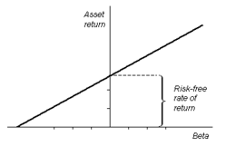The security market line, seen here in a graph, describes a relation between the beta and the asset's expected rate of return.

The CAPM is a model for pricing an individual security or portfolio. For individual securities, we make use of the security market line (SML) and its relation to expected return and systematic risk (beta) to show how the market must price individual securities in relation to their security risk class. The SML enables us to calculate the reward-to-risk ratio for any security in relation to that of the overall market. Therefore, when the expected rate of return for any security is deflated by its beta coefficient, the reward-to-risk ratio for any individual security in the market is equal to the market reward-to-risk ratio, thus:

{\frac {E(R_{i})-R_{f}}{\beta _{{i}}}}=E(R_{m})-R_{f}

The market reward-to-risk ratio is effectively the market risk premium and by rearranging the above equation and solving for $E(R_{i})~~$ , we obtain the capital asset pricing model (CAPM).

E(R_{i})=R_{f}+\beta _{{i}}(E(R_{m})-R_{f})\,

where:

$E(R_{i})~~$ is the expected return on the capital asset
$R_{f}~$ is the risk-free rate of interest such as interest arising from government bonds
$\beta _{{i}}~~$ (the beta) is the sensitivity of the expected excess asset returns to the expected excess market returns, or also $\beta _{i}={\frac {\mathrm {Cov} (R_{i},R_{m})}{\mathrm {Var} (R_{m})}}=\rho _{i,m}{\frac {\sigma _{i}}{\sigma _{m}}}$
$E(R_{m})~$ is the expected return of the market
$E(R_{m})-R_{f}~$ is sometimes known as the market premium (the difference between the expected market rate of return and the risk-free rate of return).
$E(R_{i})-R_{f}~$ is also known as the risk premium

Restated, in terms of risk premium, we find that:

E(R_{i})-R_{f}=\beta _{{i}}(E(R_{m})-R_{f})\,

which states that the individual risk premium equals the market premium times β.

Note 1: the expected market rate of return is usually estimated by measuring the arithmetic average of the historical returns on a market portfolio (e.g. S&P 500).

Note 2: the risk free rate of return used for determining the risk premium is usually the arithmetic average of historical risk free rates of return and not the current risk free rate of return.

For the full derivation see Modern portfolio theory.

Modified formula

CAPM can be modified to include size premium and specific risk. This is important for investors in privately held companies who often do not hold a well-diversified portfolio. The equation is similar to the traditional CAPM equation “with the market risk premium replaced by the product of beta times the market risk premium:”^[2]^:5

E(R_{i})=R_{f}+\beta (RP_{m})+RP_{s}+RP_{u}

"where:

E(R_{i})

is required return on security i

R_{f}

is risk-free rate

RP_{m}

is general market risk premium

RP_{s}

is risk premium for small size

RP_{u}

is risk premium due to company-specific risk factor"^[2]^:4

Security market line

The SML essentially graphs the results from the capital asset pricing model (CAPM) formula. The x-axis represents the risk (beta), and the y-axis represents the expected return. The market risk premium is determined from the slope of the SML.

The relationship between β and required return is plotted on the securities market line (SML), which shows expected return as a function of β. The intercept is the nominal risk-free rate available for the market, while the slope is the market premium, E(R_m)− R_f. The securities market line can be regarded as representing a single-factor model of the asset price, where Beta is exposure to changes in value of the Market. The equation of the SML is thus:

{\mathrm {SML}}:E(R_{i})=R_{f}+\beta _{i}(E(R_{M})-R_{f}).~

It is a useful tool in determining if an asset being considered for a portfolio offers a reasonable expected return for risk. Individual securities are plotted on the SML graph. If the security's expected return versus risk is plotted above the SML, it is undervalued since the investor can expect a greater return for the inherent risk. And a security plotted below the SML is overvalued since the investor would be accepting less return for the amount of risk assumed.

Asset pricing

Once the expected/required rate of return $E(R_{i})$ is calculated using CAPM, we can compare this required rate of return to the asset's estimated rate of return over a specific investment horizon to determine whether it would be an appropriate investment. To make this comparison, you need an independent estimate of the return outlook for the security based on either fundamental or technical analysis techniques, including P/E, M/B etc.

Assuming that the CAPM is correct, an asset is correctly priced when its estimated price is the same as the present value of future cash flows of the asset, discounted at the rate suggested by CAPM. If the estimated price is higher than the CAPM valuation, then the asset is undervalued (and overvalued when the estimated price is below the CAPM valuation).^[5] When the asset does not lie on the SML, this could also suggest mis-pricing. Since the expected return of the asset at time $t$ is $E(R_{t})={\frac {E(P_{{t+1}})-P_{t}}{P_{t}}}$ , a higher expected return than what CAPM suggests indicates that $P_{t}$ is too low (the asset is currently undervalued), assuming that at time $t+1$ the asset returns to the CAPM suggested price.^[6]

The asset price $P_{0}$ using CAPM, sometimes called the certainty equivalent pricing formula, is a linear relationship given by

P_{0}={\frac {1}{1+R_{f}}}\left[E(P_{T})-{\frac {{\mathrm {Cov}}(P_{T},R_{M})(E(R_{M})-R_{f})}{{\mathrm {Var}}(R_{M})}}\right]

where $P_T$ is the payoff of the asset or portfolio.^[5]

Asset-specific required return

The CAPM returns the asset-appropriate required return or discount rate—i.e. the rate at which future cash flows produced by the asset should be discounted given that asset's relative riskiness. Betas exceeding one signify more than average "riskiness"; betas below one indicate lower than average. Thus, a more risky stock will have a higher beta and will be discounted at a higher rate; less sensitive stocks will have lower betas and be discounted at a lower rate. Given the accepted concave utility function, the CAPM is consistent with intuition—investors (should) require a higher return for holding a more risky asset.

Since beta reflects asset-specific sensitivity to non-diversifiable, i.e. market risk, the market as a whole, by definition, has a beta of one. Stock market indices are frequently used as local proxies for the market—and in that case (by definition) have a beta of one. An investor in a large, diversified portfolio (such as a mutual fund), therefore, expects performance in line with the market.

Risk and diversification

The risk of a portfolio comprises systematic risk, also known as undiversifiable risk, and unsystematic risk which is also known as idiosyncratic risk or diversifiable risk. Systematic risk refers to the risk common to all securities—i.e. market risk. Unsystematic risk is the risk associated with individual assets. Unsystematic risk can be diversified away to smaller levels by including a greater number of assets in the portfolio (specific risks "average out"). The same is not possible for systematic risk within one market. Depending on the market, a portfolio of approximately 30–40 securities in developed markets such as the UK or US will render the portfolio sufficiently diversified such that risk exposure is limited to systematic risk only. In developing markets a larger number is required, due to the higher asset volatilities.

A rational investor should not take on any diversifiable risk, as only non-diversifiable risks are rewarded within the scope of this model. Therefore, the required return on an asset, that is, the return that compensates for risk taken, must be linked to its riskiness in a portfolio context—i.e. its contribution to overall portfolio riskiness—as opposed to its "stand alone risk." In the CAPM context, portfolio risk is represented by higher variance i.e. less predictability. In other words, the beta of the portfolio is the defining factor in rewarding the systematic exposure taken by an investor.

Efficient frontier

Main article: Efficient frontier

The (Markowitz) efficient frontier. CAL stands for the capital allocation line.

The CAPM assumes that the risk-return profile of a portfolio can be optimized—an optimal portfolio displays the lowest possible level of risk for its level of return. Additionally, since each additional asset introduced into a portfolio further diversifies the portfolio, the optimal portfolio must comprise every asset, (assuming no trading costs) with each asset value-weighted to achieve the above (assuming that any asset is infinitely divisible). All such optimal portfolios, i.e., one for each level of return, comprise the efficient frontier.

Because the unsystematic risk is diversifiable, the total risk of a portfolio can be viewed as beta.

Assumptions of CAPM

All investors:^[7]

Aim to maximize economic utilities (Asset quantities are given and fixed).
Are rational and risk-averse.
Are broadly diversified across a range of investments.
Are price takers, i.e., they cannot influence prices.
Can lend and borrow unlimited amounts under the risk free rate of interest.
Trade without transaction or taxation costs.
Deal with securities that are all highly divisible into small parcels (All assets are perfectly divisible and liquid).
Have homogeneous expectations.
Assume all information is available at the same time to all investors.

Problems of CAPM

In their 2004 review, Fama and French argue that "the failure of the CAPM in empirical tests implies that most applications of the model are invalid".^[3]

The model assumes that the variance of returns is an adequate measurement of risk. This would be implied by the assumption that returns are normally distributed, or indeed are distributed in any two-parameter way, but for general return distributions other risk measures (like coherent risk measures) will reflect the active and potential shareholders' preferences more adequately. Indeed, risk in financial investments is not variance in itself, rather it is the probability of losing: it is asymmetric in nature. Barclays Wealth have published some research on asset allocation with non-normal returns which shows that investors with very low risk tolerances should hold more cash than CAPM suggests.^[8]
The model assumes that all active and potential shareholders have access to the same information and agree about the risk and expected return of all assets (homogeneous expectations assumption).
The model assumes that the probability beliefs of active and potential shareholders match the true distribution of returns. A different possibility is that active and potential shareholders' expectations are biased, causing market prices to be informationally inefficient. This possibility is studied in the field of behavioral finance, which uses psychological assumptions to provide alternatives to the CAPM such as the overconfidence-based asset pricing model of Kent Daniel, David Hirshleifer, and Avanidhar Subrahmanyam (2001).^[9]
The model does not appear to adequately explain the variation in stock returns. Empirical studies show that low beta stocks may offer higher returns than the model would predict. Some data to this effect was presented as early as a 1969 conference in Buffalo, New York in a paper by Fischer Black, Michael Jensen, and Myron Scholes. Either that fact is itself rational (which saves the efficient-market hypothesis but makes CAPM wrong), or it is irrational (which saves CAPM, but makes the EMH wrong – indeed, this possibility makes volatility arbitrage a strategy for reliably beating the market).{H deSilva, CFA Institutes Conference Proceedings Quarterly, March 2012:46-55}{Benchmarks as Limits to Arbitrage: Understanding the Low-Volatility Anomaly. Malcolm Baker, Brendan Bradley, and Jeffrey Wurgler. people.stern.nyu.edu/jwurgler/papers/faj-benchmarks.pdf }
The model assumes that given a certain expected return, active and potential shareholders will prefer lower risk (lower variance) to higher risk and conversely given a certain level of risk will prefer higher returns to lower ones. It does not allow for active and potential shareholders who will accept lower returns for higher risk. Casino gamblers pay to take on more risk, and it is possible that some stock traders will pay for risk as well.
The model assumes that there are no taxes or transaction costs, although this assumption may be relaxed with more complicated versions of the model.
The market portfolio consists of all assets in all markets, where each asset is weighted by its market capitalization. This assumes no preference between markets and assets for individual active and potential shareholders, and that active and potential shareholders choose assets solely as a function of their risk-return profile. It also assumes that all assets are infinitely divisible as to the amount which may be held or transacted.
The market portfolio should in theory include all types of assets that are held by anyone as an investment (including works of art, real estate, human capital...) In practice, such a market portfolio is unobservable and people usually substitute a stock index as a proxy for the true market portfolio. Unfortunately, it has been shown that this substitution is not innocuous and can lead to false inferences as to the validity of the CAPM, and it has been said that due to the inobservability of the true market portfolio, the CAPM might not be empirically testable. This was presented in greater depth in a paper by Richard Roll in 1977, and is generally referred to as Roll's critique.^[10]
The model assumes economic agents optimise over a short-term horizon, and in fact investors with longer-term outlooks would optimally choose long-term inflation-linked bonds instead of short-term rates as this would be more risk-free asset to such an agent.^[11]^[12]
The model assumes just two dates, so that there is no opportunity to consume and rebalance portfolios repeatedly over time. The basic insights of the model are extended and generalized in the intertemporal CAPM (ICAPM) of Robert Merton,^[13] and the consumption CAPM (CCAPM) of Douglas Breeden and Mark Rubinstein.^[14]
CAPM assumes that all active and potential shareholders will consider all of their assets and optimize one portfolio. This is in sharp contradiction with portfolios that are held by individual shareholders: humans tend to have fragmented portfolios or, rather, multiple portfolios: for each goal one portfolio — see behavioral portfolio theory^[15] and Maslowian portfolio theory.^[16]
Empirical tests show market anomalies like the size and value effect that cannot be explained by the CAPM.^[17] For details see the Fama–French three-factor model.^[18]

References

↑ http://www.nobelprize.org/nobel_prizes/economic-sciences/laureates/1990/sharpe-lecture.pdf
1 2 3 James Chong; Yanbo Jin; Michael Phillips (April 29, 2013). "The Entrepreneur's Cost of Capital: Incorporating Downside Risk in the Buildup Method" (PDF). Retrieved 25 June 2013.
1 2 Fama, Eugene F; French, Kenneth R (Summer 2004). "The Capital Asset Pricing Model: Theory and Evidence". Journal of Economic Perspectives. 18 (3): 25–46. doi:10.1257/0895330042162430.
↑ French, Craig W. (2003). "The Treynor Capital Asset Pricing Model". Journal of Investment Management. 1 (2): 60–72. SSRN 447580.
1 2 Luenberger, David (1997). Investment Science. Oxford University Press. ISBN 978-0-19-510809-5.
↑ Bodie, Z.; Kane, A.; Marcus, A. J. (2008). Investments (7th International ed.). Boston: McGraw-Hill. p. 303. ISBN 0-07-125916-3.
↑ Arnold, Glen (2005). Corporate financial management (3. ed.). Harlow [u.a.]: Financial Times/Prentice Hall. p. 354.
↑ http://www.barclayswealth.com/Images/asset-allocation-february-2013.pdf
↑ Daniel, Kent D.; Hirshleifer, David; Subrahmanyam, Avanidhar (2001). "Overconfidence, Arbitrage, and Equilibrium Asset Pricing". Journal of Finance. 56 (3): 921–965. doi:10.1111/0022-1082.00350.
↑ Roll, R. (1977). "A Critique of the Asset Pricing Theory's Tests". Journal of Financial Economics. 4: 129–176. doi:10.1016/0304-405X(77)90009-5.
↑ http://ciber.fuqua.duke.edu/~charvey/Teaching/BA453_2006/Campbell_Viceira.pdf
↑ Campbell, J & Vicera, M "Strategic Asset Allocation: Portfolio Choice for Long Term Investors". Clarendon Lectures in Economics, 2002. ISBN 978-0-19-829694-2
↑ Merton, R.C. (1973). "An Intertemporal Capital Asset Pricing Model". Econometrica. 41 (5): 867–887. doi:10.2307/1913811.
↑ Breeden, Douglas (September 1979). "An intertemporal asset pricing model with stochastic consumption and investment opportunities". Journal of Financial Economics. 7 (3): 265–296. doi:10.1016/0304-405X(79)90016-3.
↑ Shefrin, H.; Statman, M. (2000). "Behavioral Portfolio Theory". Journal of Financial and Quantitative Analysis. 35 (2): 127–151. doi:10.2307/2676187.
↑ De Brouwer, Ph. (2009). "Maslowian Portfolio Theory: An alternative formulation of the Behavioural Portfolio Theory". Journal of Asset Management. 9 (6): 359–365. doi:10.1057/jam.2008.35.
↑ Fama, Eugene F.; French, Kenneth R. (1993). "Common Risk Factors in the Returns on Stocks and Bonds". Journal of Financial Economics. 33 (1): 3–56. doi:10.1016/0304-405X(93)90023-5.
↑ Fama, Eugene F.; French, Kenneth R. (1992). "The Cross-Section of Expected Stock Returns". Journal of Finance. 47 (2): 427–465. doi:10.2307/2329112.

Bibliography

Black, Fischer., Michael C. Jensen, and Myron Scholes (1972). The Capital Asset Pricing Model: Some Empirical Tests, pp. 79–121 in M. Jensen ed., Studies in the Theory of Capital Markets. New York: Praeger Publishers.
Fama, Eugene F. (1968). Risk, Return and Equilibrium: Some Clarifying Comments. Journal of Finance Vol. 23, No. 1, pp. 29–40.
Fama, Eugene F. and Kenneth French (1992). The Cross-Section of Expected Stock Returns. Journal of Finance, June 1992, 427–466.
French, Craig W. (2003). The Treynor Capital Asset Pricing Model, Journal of Investment Management, Vol. 1, No. 2, pp. 60–72. Available at http://www.joim.com/
French, Craig W. (2002). Jack Treynor's 'Toward a Theory of Market Value of Risky Assets' (December). Available at http://ssrn.com/abstract=628187
Lintner, John (1965). The valuation of risk assets and the selection of risky investments in stock portfolios and capital budgets, Review of Economics and Statistics, 47 (1), 13–37.
Markowitz, Harry M. (1999). The early history of portfolio theory: 1600–1960, Financial Analysts Journal, Vol. 55, No. 4
Mehrling, Perry (2005). Fischer Black and the Revolutionary Idea of Finance. Hoboken: John Wiley & Sons, Inc.
Mossin, Jan. (1966). Equilibrium in a Capital Asset Market, Econometrica, Vol. 34, No. 4, pp. 768–783.
Ross, Stephen A. (1977). The Capital Asset Pricing Model (CAPM), Short-sale Restrictions and Related Issues, Journal of Finance, 32 (177)
Rubinstein, Mark (2006). A History of the Theory of Investments. Hoboken: John Wiley & Sons, Inc.
Sharpe, William F. (1964). Capital asset prices: A theory of market equilibrium under conditions of risk, Journal of Finance, 19 (3), 425–442
Stone, Bernell K. (1970) Risk, Return, and Equilibrium: A General Single-Period Theory of Asset Selection and Capital-Market Equilibrium. Cambridge: MIT Press.
Tobin, James (1958). Liquidity preference as behavior towards risk, The Review of Economic Studies, 25
Treynor, Jack L. (1961). Market Value, Time, and Risk. Unpublished manuscript.
Treynor, Jack L. (1962). Toward a Theory of Market Value of Risky Assets. Unpublished manuscript. A final version was published in 1999, in Asset Pricing and Portfolio Performance: Models, Strategy and Performance Metrics. Robert A. Korajczyk (editor) London: Risk Books, pp. 15–22.
Mullins, David W. (1982). Does the capital asset pricing model work?, Harvard Business Review, January–February 1982, 105–113.

Financial markets

Types of markets	Primary market Secondary market Third market Fourth market

Types of stocks	Common stock Golden share Preferred stock Restricted stock Tracking stock

Share capital	Authorised capital Issued shares Shares outstanding Treasury stock

Participants	Broker-dealer Day trader Floor broker Floor trader Investor Market maker Proprietary trader Quantitative analyst Regulator Stock trader

Exchanges	Electronic communication network List of stock exchanges Opening times Multilateral trading facility Over-the-counter

Stock valuation	Alpha Arbitrage pricing theory Beta Bid–ask spread Book value Capital asset pricing model Dividend discount model Dividend yield Earnings per share Earnings yield Net asset value Security characteristic line Security market line T-model

Trading theories and strategies	Algorithmic trading Buy and hold Concentrated stock Contrarian investing Day trading Dollar cost averaging Efficient-market hypothesis Fundamental analysis Growth stock Market timing Modern portfolio theory Momentum investing Mosaic theory Pairs trade Post-modern portfolio theory Random walk hypothesis Sector rotation Style investing Swing trading Technical analysis Trend following Value investing

Related terms	Block trade Cross listing Dark liquidity Dividend Dual-listed company DuPont analysis Efficient frontier Flight-to-quality Haircut Initial public offering Margin Market anomaly Market capitalization Market depth Market manipulation Market trend Mean reversion Momentum Open outcry Public float Public offering Rally Returns-based style analysis Reverse stock split Share repurchase Short selling Slippage Speculation Stock dilution Stock market index Stock split Trade Uptick rule Volatility Voting interest Yield

Hedge funds

Investment
strategy

Arbitrage / Relative value	Capital structure arbitrage Convertible arbitrage Equity market neutral Fixed income arbitrage / Fixed-income relative-value investing Statistical arbitrage Volatility arbitrage

Event-driven	Activist shareholder Distressed securities Risk arbitrage Special situation

Directional	Convergence trade Commodity trading advisors / Managed futures account Dedicated short Global macro Long/short equity Trend following

Other	Fund of hedge funds / Multi-manager

Trading

Related
terms

Markets	Commodities Derivatives Equity Fixed income Foreign exchange Money markets Structured securities

Misc	Arbitrage pricing theory Assets under management Black–Scholes model (Greeks (finance): Delta neutral) Capital asset pricing model (Alpha / Beta / Security characteristic line) Fundamental analysis Hedge Securitization Short Taxation of private equity and hedge funds Technical analysis

Investors

Regulatory

Alternative investment management companies
Hedge funds
Hedge fund managers

This article is issued from Wikipedia - version of the 12/3/2016. The text is available under the Creative Commons Attribution/Share Alike but additional terms may apply for the media files.