Buckingham π theorem
In engineering, applied mathematics, and physics, the Buckingham π theorem is a key theorem in dimensional analysis. It is a formalization of Rayleigh's method of dimensional analysis. Loosely, the theorem states that if there is a physically meaningful equation involving a certain number n of physical variables, then the original equation can be rewritten in terms of a set of p = n − k dimensionless parameters π1, π2, ..., πp constructed from the original variables. (Here k is the number of physical dimensions involved; it is obtained as the rank of a particular matrix.)
The theorem can be seen as a scheme for nondimensionalization because it provides a method for computing sets of dimensionless parameters from the given variables, even if the form of the equation is still unknown.
Historical information
Although named for Edgar Buckingham, the π theorem was first proved by French mathematician J. Bertrand[1] in 1878. Bertrand considered only special cases of problems from electrodynamics and heat conduction, but his article contains in distinct terms all the basic ideas of the modern proof of the theorem and clearly indicates the theorem's utility for modelling physical phenomena. The technique of using the theorem (“the method of dimensions”) became widely known due to the works of Rayleigh (the first application of the π theorem in the general case[2] to the dependence of pressure drop in a pipe upon governing parameters probably dates back to 1892,[3] a heuristic proof with the use of series expansions, to 1894[4]).
Formal generalization of the π theorem for the case of arbitrarily many quantities was given first by A. Vaschy in 1892,[5] then in 1911—apparently independently—by both A. Federman[6] and D. Riabouchinsky,[7] and again in 1914 by Buckingham.[8] It was Buckingham's article that introduced the use of the symbol "πi" for the dimensionless variables (or parameters), and this is the source of the theorem's name.
Statement
More formally, the number of dimensionless terms that can be formed, p, is equal to the nullity of the dimensional matrix, and k is the rank. For experimental purposes, different systems that share the same description in terms of these dimensionless numbers are equivalent.
In mathematical terms, if we have a physically meaningful equation such as

where the qi are the n physical variables, and they are expressed in terms of k independent physical units, then the above equation can be restated as

where the πi are dimensionless parameters constructed from the qi by p = n − k dimensionless equations — the so-called Pi groups — of the form

where the exponents ai are rational numbers (they can always be taken to be integers: just raise it to a power to clear denominators).
Significance
The Buckingham π theorem provides a method for computing sets of dimensionless parameters from given variables, even if the form of the equation remains unknown. However, the choice of dimensionless parameters is not unique; Buckingham's theorem only provides a way of generating sets of dimensionless parameters and does not indicate the most "physically meaningful".
Two systems for which these parameters coincide are called similar (as with similar triangles, they differ only in scale); they are equivalent for the purposes of the equation, and the experimentalist who wants to determine the form of the equation can choose the most convenient one. Most importantly, Buckingham's theorem describes the relation between the number of variables and fundamental dimensions.
Proof
Outline
It will be assumed that the space of fundamental and derived physical units forms a vector space over the rational numbers, with the fundamental units as basis vectors, and with multiplication of physical units as the "vector addition" operation, and raising to powers as the "scalar multiplication" operation: represent a dimensional variable as the set of exponents needed for the fundamental units (with a power of zero if the particular fundamental unit is not present). For instance, the standard gravity g has units of (distance over time squared), so it is represented as the vector with respect to the basis of fundamental units (distance, time).


Making the physical units match across sets of physical equations can then be regarded as imposing linear constraints in the physical-units vector space.
Formal proof
Given a system of n dimensional variables (with physical dimensions) in k fundamental (basis) dimensions, write the dimensional matrix M, whose rows are the fundamental dimensions and whose columns are the dimensions of the variables: the (i, j)th entry is the power of the ith fundamental dimension in the jth variable. The matrix can be interpreted as taking in a combination of the dimensions of the variable quantities and giving out the dimensions of this product in fundamental dimensions. So

is the units of

A dimensionless variable is a quantity with fundamental dimensions raised to the zeroth power (the zero vector of the vector space over the fundamental dimensions), which is equivalent to the kernel of this matrix.
By the rank-nullity theorem, a system of n vectors (matrix columns) in k linearly independent dimensions (The rank of the matrix: The number of fundamental dimensions) leaves a nullity, p, satisfying (p = n − k), where the nullity is the number of extraneous dimensions which may be chosen to be dimensionless.
The dimensionless variables can always be taken to be integer combinations of the dimensional variables (by clearing denominators). There is mathematically no natural choice of dimensionless variables; some choices of dimensionless variables are more physically meaningful, and these are what are ideally used.
Examples
Speed
This example is elementary but is sufficient to demonstrate the general procedure.
Suppose a car is driving at 100 km/h; how long does it take to go 200 km?
This question considers three dimensions: distance D, time T, and velocity V. These dimensions admit a basis of two dimensions: time T and distance D. Thus there is 3 − 2 = 1 dimensionless quantity.
The dimensional matrix is

The rows correspond to the basis dimensions D and T, and the columns to the considered dimensions D, T, and V. For instance, the 3rd column (1, −1), states that the dimension V (velocity) represented by the column vector is expressible in terms of the basis dimensions as which corresponds to .
![{\displaystyle [0,0,1]}](../I/m/92abf30d73b2bf31eb4e2694477052f998996ceb.svg)
![{\displaystyle MV=[1,-1]}](../I/m/3e72638096320609fbdef0c7434a09215f3fedb8.svg)

For a dimensionless constant , we are looking for a vector such that the matrix product of M on a yields the zero vector [0,0]. In linear algebra, this vector is known as the kernel of the dimensional matrix, and it spans the nullspace of the dimensional matrix, which in this particular case is one-dimensional. The dimensional matrix as written above is in reduced row echelon form, so one can read off a kernel vector to within a multiplicative constant:

![a=[a_1,a_2,a_3]](../I/m/c0d6b4cd96414607feb0f2ab9140643897ee64b7.svg)

If the dimensional matrix were not already reduced, one could perform Gauss–Jordan elimination on the dimensional matrix to more easily determine the kernel. It follows that the dimensionless constant may be written:
- .

Since the kernel is only defined to within a multiplicative constant, if the above dimensionless constant is raised to any arbitrary power, it will yield another equivalent dimensionless constant.
Dimensional analysis has thus provided a general equation relating the three physical variables:

which may be written:

where C is one of a set of constants, such that . The actual relationship between the three variables is simply , so that the actual dimensionless equation () is written:


In other words, there is only one value of C, and it is unity. The fact that there is only a single value of C and that it is equal to unity is a level of detail not provided by the technique of dimensional analysis.
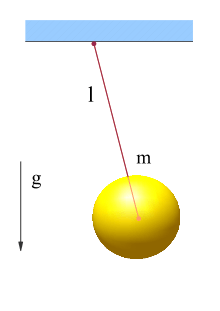
The simple pendulum
We wish to determine the period T of small oscillations in a simple pendulum. It will be assumed that it is a function of the length L, the mass M, and the acceleration due to gravity on the surface of the Earth g, which has dimensions of length divided by time squared. The model is of the form

(Note that it is written as a relation, not as a function: T isn't written here as a function of M, L, and g.)
There are 3 fundamental physical dimensions in this equation: time t, mass m, and length l, and 4 dimensional variables, T, M, L, and g. Thus we need only 4 − 3 = 1 dimensionless parameter, denoted π, and the model can be re-expressed as
where π is given by

for some values of a1, ..., a4.
The dimensions of the dimensional quantities are:

The dimensional matrix is:

(The rows correspond to the dimensions t, m, and l, and the columns to the dimensional variables T, M, L and g. For instance, the 4th column, (−2, 0, 1), states that the g variable has dimensions of .)

We are looking for a kernel vector a = [a1, a2, a3, a4] such that the matrix product of M on a yields the zero vector [0,0,0]. The dimensional matrix as written above is in reduced row echelon form, so one can read off a kernel vector within a multiplicative constant:

Were it not already reduced, one could perform Gauss–Jordan elimination on the dimensional matrix to more easily determine the kernel. It follows that the dimensionless constant may be written:

In fundamental terms:

which is dimensionless. Since the kernel is only defined to within a multiplicative constant, if the above dimensionless constant is raised to any arbitrary power, it will yield another equivalent dimensionless constant.
This example is easy because three of the dimensional quantities are fundamental units, so the last (g) is a combination of the previous. Note that if a2 were non-zero, there would be no way to cancel the M value; therefore a2 must be zero. Dimensional analysis has allowed us to conclude that the period of the pendulum is not a function of its mass. (In the 3D space of powers of mass, time, and distance, we can say that the vector for mass is linearly independent from the vectors for the three other variables. Up to a scaling factor, is the only nontrivial way to construct a vector of a dimensionless parameter.)

The model can now be expressed as:

Assuming the zeroes of f are discrete, we can say gT2/L = Cn, where Cn is the nth zero of the function f. If there is only one zero, then gT2/L = C. It requires more physical insight or an experiment to show that there is indeed only one zero and that the constant is in fact given by C = 4π2.
For large oscillations of a pendulum, the analysis is complicated by an additional dimensionless parameter, the maximum swing angle. The above analysis is a good approximation as the angle approaches zero.
See also
- Blast wave
- Dimensional analysis
- Dimensionless quantity
- Natural units
- Nondimensionalization
- Similitude (model)
- Rayleigh's method of dimensional analysis
References
Notes
- ↑ Bertrand, J. (1878). "Sur l'homogénéité dans les formules de physique". Comptes rendus. 86 (15): 916–920.
- ↑ When in applying the pi–theorem there arises an arbitrary function of dimensionless numbers.
- ↑ Rayleigh (1892). "On the question of the stability of the flow of liquids". Philosophical magazine. 34: 59–70. doi:10.1080/14786449208620167.
- ↑ Second edition of ``The Theory of Sound’’(Strutt, John William (1896). The Theory of Sound. 2. Macmillan.).
- ↑ Quotes from Vaschy’s article with his statement of the pi–theorem can be found in: Macagno, E. O. (1971). "Historico-critical review of dimensional analysis". Journal of the Franklin Institute. 292 (6): 391–402. doi:10.1016/0016-0032(71)90160-8.
- ↑ Федерман, А. (1911). "О некоторых общих методах интегрирования уравнений с частными производными первого порядка". Известия Санкт-Петербургского политехнического института императора Петра Великого. Отдел техники, естествознания и математики. 16 (1): 97–155. (Federman A., On some general methods of integration of first-order partial differential equations, Proceedings of the Saint-Petersburg polytechnic institute. Section of technics, natural science, and mathematics)
- ↑ Riabouchinsky, D. (1911). "Мéthode des variables de dimension zéro et son application en aérodynamique". L'Aérophile: 407–408.
- ↑ Original text of Buckingham’s article in Physical Review
Exposition
- Hanche-Olsen, Harald (2004). "Buckingham's pi-theorem" (PDF). NTNU. Retrieved April 9, 2007.
- Hart, George W. (March 1, 1995). Multidimensional Analysis: Algebras and Systems for Science and Engineering. Springer-Verlag. ISBN 0-387-94417-6.
- Kline, Stephen J. (1986). Similitude and Approximation Theory. Springer-Verlag, New York. ISBN 0-387-16518-5.
- Wan, Frederic Y.M. (1989). Mathematical Models and their Analysis. Harper & Row Publishers, New York. ISBN 0-06-046902-1.
- Vignaux, G.A. (1991). "Dimensional analysis in data modelling" (PDF). Victoria University of Wellington. Retrieved December 15, 2005.
- Mike Sheppard, 2007 Systematic Search for Expressions of Dimensionless Constants using the NIST database of Physical Constants
- Gibbings, J.C. (2011). Dimensional Analysis. Springer. ISBN 1-84996-316-9.
Original sources
- Vaschy, A. (1892). "Sur les lois de similitude en physique". Annales Télégraphiques. 19: 25–28.
- Buckingham, E. (1914). "On physically similar systems; illustrations of the use of dimensional equations". Physical Review. 4 (4): 345–376. Bibcode:1914PhRv....4..345B. doi:10.1103/PhysRev.4.345.
- Buckingham, E. (1915). "The principle of similitude". Nature. 96 (2406): 396–397. Bibcode:1915Natur..96..396B. doi:10.1038/096396d0.
- Buckingham, E. (1915). "Model experiments and the forms of empirical equations". Transactions of the American Society of Mechanical Engineers. 37: 263–296.
- Taylor, Sir G. (1950). "The Formation of a Blast Wave by a Very Intense Explosion. I. Theoretical Discussion". Proceedings of the Royal Society A. 201 (1065): 159–174. Bibcode:1950RSPSA.201..159T. doi:10.1098/rspa.1950.0049.
- Taylor, Sir G. (1950). "The Formation of a Blast Wave by a Very Intense Explosion. II. The Atomic Explosion of 1945". Proceedings of the Royal Society A. 201 (1065): 175–186. Bibcode:1950RSPSA.201..175T. doi:10.1098/rspa.1950.0050.