Bisection bandwidth
In computer networking, if the network is bisected into two partitions, the bisection bandwidth of a network topology is the bandwidth available between the two partitions.[1] Bisection should be done in such a way that the bandwidth between two partitions is minimum.[2] Bisection bandwidth gives the true bandwidth available in the entire system. Bisection bandwidth accounts for the bottleneck bandwidth of entire network. Therefore bisection bandwidth represents bandwidth characteristics of the network better than any other metric.
Bisection bandwidth calculations[2]
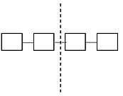
For a linear array with n nodes bisection bandwidth is one link bandwidth. For linear array only one link needs to be broken to bisect the network into two partitions.
For ring topology with n nodes two links should be broken to bisect the network, so bisection bandwidth becomes bandwidth of two links.

For tree topology with n nodes can be bisected at the root by breaking one link, so bisection bandwidth is one link bandwidth.

For Mesh topology with n nodes, links should be broken to bisect the network, so bisection bandwidth is bandwidth of links.


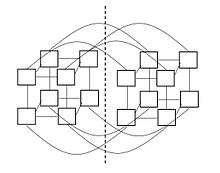
For Hyper-cube topology with n nodes, n/2 links should be broken to bisect the network, so bisection bandwidth is bandwidth of n/2 links.
Significance of bisection bandwidth
Theoretical support for the importance of this measure of network performance was developed in the PhD research of Clark Thomborson (formerly Clark Thompson).[3] Thomborson proved that important algorithms for sorting, Fast Fourier transformation, and matrix-matrix multiplication become communication-limited—as opposed to CPU-limited or memory-limited—on computers with insufficient bisection width. F. Thomson Leighton's PhD research[4] tightened Thomborson's loose bound [5] on the bisection width of a computationally-important variant of the De Bruijn graph known as the shuffle-exchange graph. Based on Bill Dally's analysis of latency, average case throughput, and hot-spot throughput of m-ary n-cube networks[2] for various m, It can be observed that low-dimensional networks,in comparison to high-dimensional networks (e.g., binary n-cubes) with the same bisection width (e.g., tori), have reduced latency and higher hot-spot throughput.[6]
References
- ↑ John L. Hennessy and David A. Patterson (2003). Computer Architecture: A Quantitative Approach (Third ed.). Morgan Kaufmann Publishers, Inc. p. 789. ISBN 1-55860-596-7.
- 1 2 3 Solihin, Yan (2016). Fundamentals of parallel multicore architecture. CRC Press. pp. 371–381. ISBN 9781482211191.
- ↑ C. D. Thompson (1980). A complexity theory for VLSI (PDF) (Thesis). Carnegie-Mellon University.
- ↑ F. Thomson Leighton (1983). Complexity Issues in VLSI: Optimal layouts for the shuffle-exchange graph and other networks (Thesis). MIT Press. ISBN 0-262-12104-2.
- ↑ Clark Thompson (1979). Area-time complexity for VLSI. Proc. Caltech Conf. on VLSI Systems and Computations. pp. 81–88.
- ↑ Bill Dally (1990). "Performance analysis of k-ary n-cube interconnection networks". IEEE Transactions on Computers. 39 (6). doi:10.1109/12.53599.