Bipolar coordinates
Bipolar coordinates are a two-dimensional orthogonal coordinate system. There are two commonly defined types of bipolar coordinates.[1] The first is based on the Apollonian circles. The curves of constant σ and of τ are circles that intersect at right angles. The coordinates have two foci F1 and F2, which are generally taken to be fixed at (−a, 0) and (a, 0), respectively, on the x-axis of a Cartesian coordinate system. The second system is two-center bipolar coordinates. There is also a third coordinate system that is based on two poles (biangular coordinates).
The term "bipolar" is sometimes used to describe other curves having two singular points (foci), such as ellipses, hyperbolas, and Cassini ovals. However, the term bipolar coordinates is reserved for the coordinates described here, and never used to describe coordinates associated with those other curves, such as elliptic coordinates.

Definition
The most common definition of bipolar coordinates (σ, τ) is


where the σ-coordinate of a point P equals the angle F1 P F2 and the τ-coordinate equals the natural logarithm of the ratio of the distances d1 and d2 to the foci

(Recall that F1 and F2 are located at (−a, 0) and (a, 0), respectively.) Equivalently

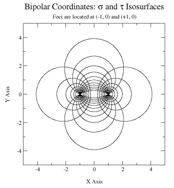
Curves of constant σ and τ


The curves of constant σ correspond to non-concentric circles

that intersect at the two foci. The centers of the constant-σ circles lie on the y-axis. Circles of positive σ are centered above the x-axis, whereas those of negative σ lie below the axis. As the magnitude |σ| increases, the radius of the circles decreases and the center approaches the origin (0, 0), which is reached when |σ| = π/2, its maximum value.
The curves of constant are non-intersecting circles of different radii


that surround the foci but again are not concentric. The centers of the constant-τ circles lie on the x-axis. The circles of positive τ lie in the right-hand side of the plane (x > 0), whereas the circles of negative τ lie in the left-hand side of the plane (x < 0). The τ = 0 curve corresponds to the y-axis (x = 0). As the magnitude of τ increases, the radius of the circles decreases and their centers approach the foci.
Reciprocal relations
The passage from the Cartesian coordinates towards the bipolar coordinates can be done via the following formulas:

and

We notice also those two remarkable identities:

and

Scale factors
The scale factors for the bipolar coordinates (σ, τ) are equal

Thus, the infinitesimal area element equals

and the Laplacian is given by

Other differential operators such as and can be expressed in the coordinates (σ, τ) by substituting the scale factors into the general formulae found in orthogonal coordinates.


Applications
The classic applications of bipolar coordinates are in solving partial differential equations, e.g., Laplace's equation or the Helmholtz equation, for which bipolar coordinates allow a separation of variables. A typical example would be the electric field surrounding two parallel cylindrical conductors.
Extension to 3-dimensions
Bipolar coordinates form the basis for several sets of three-dimensional orthogonal coordinates. The bipolar cylindrical coordinates are produced by projecting in the z-direction. The bispherical coordinates are produced by rotating the bipolar coordinates about the -axis, i.e., the axis connecting the foci, whereas the toroidal coordinates are produced by rotating the bipolar coordinates about the y-axis, i.e., the axis separating the foci.

References
- ↑ Eric W. Weisstein, Concise Encyclopedia of Mathematics CD-ROM, Bipolar Coordinates, CD-ROM edition 1.0, May 20, 1999 Archived December 12, 2007, at the Wayback Machine.
- ↑ Polyanin, Andrei Dmitrievich (2002). Handbook of linear partial differential equations for engineers and scientists. CRC Press. p. 476. ISBN 1-58488-299-9.
- ↑ Happel, John; Brenner, Howard (1983). Low Reynolds number hydrodynamics: with special applications to particulate media. Mechanics of fluids and transport processes. 1. Springer. p. 497. ISBN 978-90-247-2877-0.
- H. Bateman "Spheroidal and bipolar coordinates", Duke Mathematical Journal 4 (1938), no. 1, 39–50
- Hazewinkel, Michiel, ed. (2001), "Bipolar coordinates", Encyclopedia of Mathematics, Springer, ISBN 978-1-55608-010-4
- Lockwood, E. H. "Bipolar Coordinates." Chapter 25 in A Book of Curves. Cambridge, England: Cambridge University Press, pp. 186–190, 1967.
- Korn GA and Korn TM. (1961) Mathematical Handbook for Scientists and Engineers, McGraw-Hill.