Analysis of algorithms

Graphs of number of operations, N vs input size, n for common complexities, assuming a coefficient of 1

In computer science, the analysis of algorithms is the determination of the amount of resources (such as time and storage) necessary to execute them. Most algorithms are designed to work with inputs of arbitrary length. Usually, the efficiency or running time of an algorithm is stated as a function relating the input length to the number of steps (time complexity) or storage locations (space complexity).

The term "analysis of algorithms" was coined by Donald Knuth.^[1] Algorithm analysis is an important part of a broader computational complexity theory, which provides theoretical estimates for the resources needed by any algorithm which solves a given computational problem. These estimates provide an insight into reasonable directions of search for efficient algorithms.

In theoretical analysis of algorithms it is common to estimate their complexity in the asymptotic sense, i.e., to estimate the complexity function for arbitrarily large input. Big O notation, Big-omega notation and Big-theta notation are used to this end. For instance, binary search is said to run in a number of steps proportional to the logarithm of the length of the sorted list being searched, or in O(log(n)), colloquially "in logarithmic time". Usually asymptotic estimates are used because different implementations of the same algorithm may differ in efficiency. However the efficiencies of any two "reasonable" implementations of a given algorithm are related by a constant multiplicative factor called a hidden constant.

Exact (not asymptotic) measures of efficiency can sometimes be computed but they usually require certain assumptions concerning the particular implementation of the algorithm, called model of computation. A model of computation may be defined in terms of an abstract computer, e.g., Turing machine, and/or by postulating that certain operations are executed in unit time. For example, if the sorted list to which we apply binary search has n elements, and we can guarantee that each lookup of an element in the list can be done in unit time, then at most log₂ n + 1 time units are needed to return an answer.

Cost models

Time efficiency estimates depend on what we define to be a step. For the analysis to correspond usefully to the actual execution time, the time required to perform a step must be guaranteed to be bounded above by a constant. One must be careful here; for instance, some analyses count an addition of two numbers as one step. This assumption may not be warranted in certain contexts. For example, if the numbers involved in a computation may be arbitrarily large, the time required by a single addition can no longer be assumed to be constant.

Two cost models are generally used:^[2]^[3]^[4]^[5]^[6]

the uniform cost model, also called uniform-cost measurement (and similar variations), assigns a constant cost to every machine operation, regardless of the size of the numbers involved
the logarithmic cost model, also called logarithmic-cost measurement (and similar variations), assigns a cost to every machine operation proportional to the number of bits involved

The latter is more cumbersome to use, so it's only employed when necessary, for example in the analysis of arbitrary-precision arithmetic algorithms, like those used in cryptography.

A key point which is often overlooked is that published lower bounds for problems are often given for a model of computation that is more restricted than the set of operations that you could use in practice and therefore there are algorithms that are faster than what would naively be thought possible.^[7]

Run-time analysis

Run-time analysis is a theoretical classification that estimates and anticipates the increase in running time (or run-time) of an algorithm as its input size (usually denoted as n) increases. Run-time efficiency is a topic of great interest in computer science: A program can take seconds, hours or even years to finish executing, depending on which algorithm it implements (see also performance analysis, which is the analysis of an algorithm's run-time in practice).

Shortcomings of empirical metrics

Since algorithms are platform-independent (i.e. a given algorithm can be implemented in an arbitrary programming language on an arbitrary computer running an arbitrary operating system), there are significant drawbacks to using an empirical approach to gauge the comparative performance of a given set of algorithms.

Take as an example a program that looks up a specific entry in a sorted list of size n. Suppose this program were implemented on Computer A, a state-of-the-art machine, using a linear search algorithm, and on Computer B, a much slower machine, using a binary search algorithm. Benchmark testing on the two computers running their respective programs might look something like the following:

n (list size)	Computer A run-time (in nanoseconds)	Computer B run-time (in nanoseconds)
16	8	100,000
63	32	150,000
250	125	200,000
1,000	500	250,000

Based on these metrics, it would be easy to jump to the conclusion that Computer A is running an algorithm that is far superior in efficiency to that of Computer B. However, if the size of the input-list is increased to a sufficient number, that conclusion is dramatically demonstrated to be in error:

n (list size)	Computer A run-time (in nanoseconds)	Computer B run-time (in nanoseconds)
16	8	100,000
63	32	150,000
250	125	200,000
1,000	500	250,000
...	...	...
1,000,000	500,000	500,000
4,000,000	2,000,000	550,000
16,000,000	8,000,000	600,000
...	...	...
63,072 × 10¹²	31,536 × 10¹² ns, or 1 year	1,375,000 ns, or 1.375 milliseconds

Computer A, running the linear search program, exhibits a linear growth rate. The program's run-time is directly proportional to its input size. Doubling the input size doubles the run time, quadrupling the input size quadruples the run-time, and so forth. On the other hand, Computer B, running the binary search program, exhibits a logarithmic growth rate. Quadrupling the input size only increases the run time by a constant amount (in this example, 50,000 ns). Even though Computer A is ostensibly a faster machine, Computer B will inevitably surpass Computer A in run-time because it's running an algorithm with a much slower growth rate.

Orders of growth

Main article: Big O notation

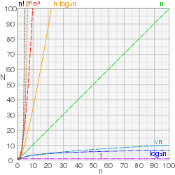
Informally, an algorithm can be said to exhibit a growth rate on the order of a mathematical function if beyond a certain input size n, the function $f(n)$ times a positive constant provides an upper bound or limit for the run-time of that algorithm. In other words, for a given input size n greater than some n₀ and a constant c, the running time of that algorithm will never be larger than $c\times f(n)$ . This concept is frequently expressed using Big O notation. For example, since the run-time of insertion sort grows quadratically as its input size increases, insertion sort can be said to be of order O(n²).

Big O notation is a convenient way to express the worst-case scenario for a given algorithm, although it can also be used to express the average-case — for example, the worst-case scenario for quicksort is O(n²), but the average-case run-time is $O (n log n)$ .

Empirical orders of growth

Assuming the execution time follows power rule, $t \approx k n a$ , the coefficient a can be found ^[8] by taking empirical measurements of run time $\{t_{1},t_{2}\}$ at some problem-size points $\{n_{1},n_{2}\}$ , and calculating $t_{2}/t_{1}=(n_{2}/n_{1})^{a}$ so that $a=\log(t_{2}/t_{1})/\log(n_{2}/n_{1})$ . In other words, this measures the slope of the empirical line on the log–log plot of execution time vs. problem size, at some size point. If the order of growth indeed follows the power rule (and so the line on log–log plot is indeed a straight line), the empirical value of a will stay constant at different ranges, and if not, it will change (and the line is a curved line) - but still could serve for comparison of any two given algorithms as to their empirical local orders of growth behaviour. Applied to the above table:

n (list size)	Computer A run-time (in nanoseconds)	Local order of growth (n^_)	Computer B run-time (in nanoseconds)	Local order of growth (n^_)
15	7		100,000
65	32	1.04	150,000	0.28
250	125	1.01	200,000	0.21
1,000	500	1.00	250,000	0.16
...	...		...
1,000,000	500,000	1.00	500,000	0.10
4,000,000	2,000,000	1.00	550,000	0.07
16,000,000	8,000,000	1.00	600,000	0.06
...	...		...

It is clearly seen that the first algorithm exhibits a linear order of growth indeed following the power rule. The empirical values for the second one are diminishing rapidly, suggesting it follows another rule of growth and in any case has much lower local orders of growth (and improving further still), empirically, than the first one.

Evaluating run-time complexity

The run-time complexity for the worst-case scenario of a given algorithm can sometimes be evaluated by examining the structure of the algorithm and making some simplifying assumptions. Consider the following pseudocode:

1    get a positive integer from input
2    if n > 10
3        print "This might take a while..."
4    for i = 1 to n
5        for j = 1 to i
6            print i * j
7    print "Done!"

A given computer will take a discrete amount of time to execute each of the instructions involved with carrying out this algorithm. The specific amount of time to carry out a given instruction will vary depending on which instruction is being executed and which computer is executing it, but on a conventional computer, this amount will be deterministic.^[9] Say that the actions carried out in step 1 are considered to consume time T₁, step 2 uses time T₂, and so forth.

In the algorithm above, steps 1, 2 and 7 will only be run once. For a worst-case evaluation, it should be assumed that step 3 will be run as well. Thus the total amount of time to run steps 1-3 and step 7 is:

T_{1}+T_{2}+T_{3}+T_{7}.\,

The loops in steps 4, 5 and 6 are trickier to evaluate. The outer loop test in step 4 will execute ( n + 1 ) times (note that an extra step is required to terminate the for loop, hence n + 1 and not n executions), which will consume T₄( n + 1 ) time. The inner loop, on the other hand, is governed by the value of i, which iterates from 1 to i. On the first pass through the outer loop, j iterates from 1 to 1: The inner loop makes one pass, so running the inner loop body (step 6) consumes T₆ time, and the inner loop test (step 5) consumes 2T₅ time. During the next pass through the outer loop, j iterates from 1 to 2: the inner loop makes two passes, so running the inner loop body (step 6) consumes 2T₆ time, and the inner loop test (step 5) consumes 3T₅ time.

Altogether, the total time required to run the inner loop body can be expressed as an arithmetic progression:

T_{6}+2T_{6}+3T_{6}+\cdots +(n-1)T_{6}+nT_{6}

which can be factored^[10] as

T_{6}\left[1+2+3+\cdots +(n-1)+n\right]=T_{6}\left[{\frac {1}{2}}(n^{2}+n)\right]

The total time required to run the outer loop test can be evaluated similarly:

{\begin{aligned}&2T_{5}+3T_{5}+4T_{5}+\cdots +(n-1)T_{5}+nT_{5}+(n+1)T_{5}\\=\ &T_{5}+2T_{5}+3T_{5}+4T_{5}+\cdots +(n-1)T_{5}+nT_{5}+(n+1)T_{5}-T_{5}\end{aligned}}

which can be factored as

{\begin{aligned}&T_{5}\left[1+2+3+\cdots +(n-1)+n+(n+1)\right]-T_{5}\\=&\left[{\frac {1}{2}}(n^{2}+n)\right]T_{5}+(n+1)T_{5}-T_{5}\\=&T_{5}\left[{\frac {1}{2}}(n^{2}+n)\right]+nT_{5}\\=&\left[{\frac {1}{2}}(n^{2}+3n)\right]T_{5}\end{aligned}}

Therefore, the total running time for this algorithm is:

f(n)=T_{1}+T_{2}+T_{3}+T_{7}+(n+1)T_{4}+\left[{\frac {1}{2}}(n^{2}+n)\right]T_{6}+\left[{\frac {1}{2}}(n^{2}+3n)\right]T_{5}

which reduces to

f(n)=\left[{\frac {1}{2}}(n^{2}+n)\right]T_{6}+\left[{\frac {1}{2}}(n^{2}+3n)\right]T_{5}+(n+1)T_{4}+T_{1}+T_{2}+T_{3}+T_{7}

As a rule-of-thumb, one can assume that the highest-order term in any given function dominates its rate of growth and thus defines its run-time order. In this example, n² is the highest-order term, so one can conclude that f(n) = O(n²). Formally this can be proven as follows:

Prove that $\left[{\frac {1}{2}}(n^{2}+n)\right]T_{6}+\left[{\frac {1}{2}}(n^{2}+3n)\right]T_{5}+(n+1)T_{4}+T_{1}+T_{2}+T_{3}+T_{7}\leq cn^{2},\ n\geq n_{0}$

${\begin{aligned}&\left[{\frac {1}{2}}(n^{2}+n)\right]T_{6}+\left[{\frac {1}{2}}(n^{2}+3n)\right]T_{5}+(n+1)T_{4}+T_{1}+T_{2}+T_{3}+T_{7}\\\leq &(n^{2}+n)T_{6}+(n^{2}+3n)T_{5}+(n+1)T_{4}+T_{1}+T_{2}+T_{3}+T_{7}\ ({\text{for }}n\geq 0)\end{aligned}}$

Let k be a constant greater than or equal to [T₁..T₇]

${\begin{aligned}&T_{6}(n^{2}+n)+T_{5}(n^{2}+3n)+(n+1)T_{4}+T_{1}+T_{2}+T_{3}+T_{7}\leq k(n^{2}+n)+k(n^{2}+3n)+kn+5k\\=&2kn^{2}+5kn+5k\leq 2kn^{2}+5kn^{2}+5kn^{2}\ ({\text{for }}n\geq 1)=12kn^{2}\end{aligned}}$

Therefore $\left[{\frac {1}{2}}(n^{2}+n)\right]T_{6}+\left[{\frac {1}{2}}(n^{2}+3n)\right]T_{5}+(n+1)T_{4}+T_{1}+T_{2}+T_{3}+T_{7}\leq cn^{2},n\geq n_{0}{\text{ for }}c=12k,n_{0}=1$

A more elegant approach to analyzing this algorithm would be to declare that [T₁..T₇] are all equal to one unit of time, in a system of units chosen so that one unit is greater than or equal to the actual times for these steps. This would mean that the algorithm's running time breaks down as follows:^[11]

$4+\sum _{i=1}^{n}i\leq 4+\sum _{i=1}^{n}n=4+n^{2}\leq 5n^{2}\ ({\text{for }}n\geq 1)=O(n^{2}).$

Growth rate analysis of other resources

The methodology of run-time analysis can also be utilized for predicting other growth rates, such as consumption of memory space. As an example, consider the following pseudocode which manages and reallocates memory usage by a program based on the size of a file which that program manages:

while (file still open)
    let n = size of file
    for every 100,000 kilobytes of increase in file size
        double the amount of memory reserved

In this instance, as the file size n increases, memory will be consumed at an exponential growth rate, which is order O(2ⁿ). This is an extremely rapid and most likely unmanageable growth rate for consumption of memory resources.

Relevance

Algorithm analysis is important in practice because the accidental or unintentional use of an inefficient algorithm can significantly impact system performance. In time-sensitive applications, an algorithm taking too long to run can render its results outdated or useless. An inefficient algorithm can also end up requiring an uneconomical amount of computing power or storage in order to run, again rendering it practically useless.

Constant factors

Analysis of algorithms typically focuses on the asymptotic performance, particularly at the elementary level, but in practical applications constant factors are important, and real-world data is in practice always limited in size. The limit is typically the size of addressable memory, so on 32-bit machines 2³² = 4 GiB (greater if segmented memory is used) and on 64-bit machines 2⁶⁴ = 16 EiB. Thus given a limited size, an order of growth (time or space) can be replaced by a constant factor, and in this sense all practical algorithms are O(1) for a large enough constant, or for small enough data.

This interpretation is primarily useful for functions that grow extremely slowly: (binary) iterated logarithm (log^*) is less than 5 for all practical data (2⁶⁵⁵³⁶ bits); (binary) log-log (log log n) is less than 6 for virtually all practical data (2⁶⁴ bits); and binary log (log n) is less than 64 for virtually all practical data (2⁶⁴ bits). An algorithm with non-constant complexity may nonetheless be more efficient than an algorithm with constant complexity on practical data if the overhead of the constant time algorithm results in a larger constant factor, e.g., one may have $K>k\log \log n$ so long as $K/k>6$ and $n<2^{{2^{6}}}=2^{{64}}$ .

For large data linear or quadratic factors cannot be ignored, but for small data an asymptotically inefficient algorithm may be more efficient. This is particularly used in hybrid algorithms, like Timsort, which use an asymptotically efficient algorithm (here merge sort, with time complexity $n\log n$ ), but switch to an asymptotically inefficient algorithm (here insertion sort, with time complexity $n^{2}$ ) for small data, as the simpler algorithm is faster on small data.

Notes

↑ Donald Knuth, Recent News
↑ Alfred V. Aho; John E. Hopcroft; Jeffrey D. Ullman (1974). The design and analysis of computer algorithms. Addison-Wesley Pub. Co. , section 1.3
↑ Juraj Hromkovič (2004). Theoretical computer science: introduction to Automata, computability, complexity, algorithmics, randomization, communication, and cryptography. Springer. pp. 177–178. ISBN 978-3-540-14015-3.
↑ Giorgio Ausiello (1999). Complexity and approximation: combinatorial optimization problems and their approximability properties. Springer. pp. 3–8. ISBN 978-3-540-65431-5.
↑ Wegener, Ingo (2005), Complexity theory: exploring the limits of efficient algorithms, Berlin, New York: Springer-Verlag, p. 20, ISBN 978-3-540-21045-0
↑ Robert Endre Tarjan (1983). Data structures and network algorithms. SIAM. pp. 3–7. ISBN 978-0-89871-187-5.
↑ Examples of the price of abstraction?, cstheory.stackexchange.com
↑ How To Avoid O-Abuse and Bribes, at the blog "Gödel’s Lost Letter and P=NP" by R. J. Lipton, professor of Computer Science at Georgia Tech, recounting idea by Robert Sedgewick
↑ However, this is not the case with a quantum computer
↑ It can be proven by induction that $1+2+3+\cdots +(n-1)+n={\frac {n(n+1)}{2}}$
↑ This approach, unlike the above approach, neglects the constant time consumed by the loop tests which terminate their respective loops, but it is trivial to prove that such omission does not affect the final result

References

Cormen, Thomas H.; Leiserson, Charles E.; Rivest, Ronald L. & Stein, Clifford (2001). Introduction to Algorithms. Chapter 1: Foundations (Second ed.). Cambridge, MA: MIT Press and McGraw-Hill. pp. 3–122. ISBN 0-262-03293-7.
Sedgewick, Robert (1998). Algorithms in C, Parts 1-4: Fundamentals, Data Structures, Sorting, Searching (3rd ed.). Reading, MA: Addison-Wesley Professional. ISBN 978-0-201-31452-6.
Knuth, Donald. The Art of Computer Programming. Addison-Wesley.
Greene, Daniel A.; Knuth, Donald E. (1982). Mathematics for the Analysis of Algorithms (Second ed.). Birkhäuser. ISBN 3-7643-3102-X.
Goldreich, Oded (2010). Computational Complexity: A Conceptual Perspective. Cambridge University Press. ISBN 978-0-521-88473-0.

Major fields of computer science

Note: This template roughly follows the 2012 ACM Computing classification.

Hardware	Printed circuit board Peripheral Integrated circuit Very-large-scale integration Energy consumption Electronic design automation

Computer systems organization	Computer architecture Embedded system Real-time computing Dependability

Networks	Network architecture Network protocol Network components Network scheduler Network performance evaluation Network service

Software organization	Interpreter Middleware Virtual machine Operating system Software quality

Software notations and tools	Programming paradigm Programming language Compiler Domain-specific language Modeling language Software framework Integrated development environment Software configuration management Software library Software repository

Software development	Software development process Requirements analysis Software design Software construction Software deployment Software maintenance Programming team Open-source model

Theory of computation	Model of computation Formal language Automata theory Computational complexity theory Logic Semantics

Algorithms	Algorithm design Analysis of algorithms Randomized algorithm Computational geometry

Mathematics of computing	Discrete mathematics Probability Statistics Mathematical software Information theory Mathematical analysis Numerical analysis

Information systems	Database management system Information storage systems Enterprise information system Social information systems Geographic information system Decision support system Process control system Multimedia information system Data mining Digital library Computing platform Digital marketing World Wide Web Information retrieval

Security	Cryptography Formal methods Security services Intrusion detection system Hardware security Network security Information security Application security

Human–computer interaction	Interaction design Social computing Ubiquitous computing Visualization Accessibility

Concurrency	Concurrent computing Parallel computing Distributed computing Multithreading Multiprocessing

Artificial intelligence	Natural language processing Knowledge representation and reasoning Computer vision Automated planning and scheduling Search methodology Control method Philosophy of artificial intelligence Distributed artificial intelligence

Machine learning	Supervised learning Unsupervised learning Reinforcement learning Multi-task learning Machine learning algorithms Cross-validation

Graphics	Animation Rendering Image manipulation Graphics processing unit Mixed reality Virtual reality Image compression Solid modeling

Applied computing	E-commerce Enterprise software Computational mathematics Computational physics Computational chemistry Computational biology Computational social science Computational engineering Computational healthcare Digital art Electronic publishing Cyberwarfare Electronic voting Video game Word processing Operations research Educational technology Document management

Computer science portal

This article is issued from Wikipedia - version of the 12/1/2016. The text is available under the Creative Commons Attribution/Share Alike but additional terms may apply for the media files.